Project Evaluation

Once projects reach the selected lists, the next phase is project evaluation. This phase

will determine which projects can advance to detail design and which will require a

more detailed evaluation in preliminary development.

Projects that can advance directly to design phase meet the following criteria:

• No additional right-of-way (permanent or temporary) will be required to accomplish the work and there will be no adverse effect on abutting real properties.

• No major changes in the operation of access points, traffic volumes, traffic flows, vehicle mix, or traffic patterns.

• No involvement with a live stream or an intermittent stream having significant year – round pools, upstream or downstream, in the immediate vicinity.

• No involvement with a historic site.

Examples of these types of improvement are:

• Restoration and/or reconstruction of existing pavement surfaces

• Modernization of an existing facility by adding or widening shoulders

• Modernization of existing facilities by adding auxiliary lanes or pavement widening to accomplish a localized purpose (weaving, climbing, speed change, protected turn, etc.)

• Intersection improvements

• Reconstruction or rehabilitation of existing grade separation structures

• Reconstruction or rehabilitation of existing stream crossings which do not involve any modification of a live stream or otherwise affect the water quality

• Landscaping or rest area upgrading projects

• Lighting, signing, pavement marking, signalization, freeway surveillance and control systems, railroad protective devices, etc.

• Minor safety-type improvements, such as guiderail replacement or installation of breakaway sign hardware

• Outdoor advertising control programs

• Bicycle or pedestrian facilities provided within existing right-of-way

All projects that do not fall into the above categories must undergo additional evaluation in a preliminary development phase.

SQUARE

Foundations and Floors

Floors may seem to be the simplest of the challenges facing a new builder, but the importance of establishing a firm, sound, dependable connection between a house, the foundation, and the earth cannot be overstated. Everything rests, quite literally, on the quality of the foundation and fram­ing work done in the first few days or so after the concrete contractor has left. Our first house, in coastal Oregon, had a concrete foundation made from beach sand. Sixty years of wind and rain had washed much of that sand back toward the beach, leaving us with a shaky, tilted floor that wasn’t even bolted to the foundation.

Know the Foundation Fundamentals

Take a deep breath. Having found and purchased a lot, bought or drawn up the plans, obtained the permits, cleared the land, run power to the site, and completed the necessary grading, drainage, and excavation work, you’re finally ready to begin working on the foundation. You’ve already come a long way.

Whenever I think about foundations, I can’t help but recall being told as a child, “You’re on your feet most of the day, so wear good shoes.” A foundation is like a pair of shoes—quality makes all the difference. Walk around all day in poor shoes and your whole body feels lousy. Build a house on a poor founda­tion and the entire house is unstable.

Подпись: STEP BY STEPПодпись: 1 Form and Pour the Footings p. 52 2 Build the Foundation Walls p. 53 3 Backfill around the Foundation p. 54 4 Attach the Sills p. 55 5 Build Midspan Support for Joists p. 60 6 Install the Joists p. 65 7 Install Extra Joists and Blocking p. 69 8 Install the Floor Sheathing p. 71 SQUAREThere are quite a few foundations that can be used for houses. The three major types—slabs, crawl spaces, and full basements—are discussed in the sidebar on pp. 50—51. Because many houses have a crawl-space foundation, we’ll cover the step-by-step process for this type shortly. The main parts of this

Подпись: и їм їм їм и їм їм їм їм їм їм їм їм їм їм їм їм їм їм и їм їм їм їм їм їм їм їм їм їм їм їм їм и їм їм їм їм їм їм їм їм їм їм їм їм їм їм и їм їм їм їм їм їм їм їм їм їм їм їм їм и їм їм їм їм їм їм їм їм і FOUNDATION AND FRAMING SQUAREAll foundations need proper drainage. In addition to installing drainpipe around the footings, make sure that the finished grade slopes away from the house. If gutters and downspouts are installed, use elbows and splash plates to direct runoff away from foundation walls.

SQUARE

foundation are shown in the illustration above. However, if you’re planning to build a house, it’s a good idea to consider all your foundation options. Talk to builders and foundation sub­contractors in your area to find out which foun­dations and special site conditions to consider.

If you’re building a crawl-space foundation, as we did here, find out about the ventilation requirements. In most areas, vents are required in crawl-space foundations. In some areas, codes have been updated to allow for an unvented crawl space (see the sidebar on the facing page).

Clay can cause problems

Local soil conditions have a lot to do with choosing and constructing a foundation. Extra care must be taken when building on clay-rich soils, which exist in many parts of the country. Clay expands when saturated with moisture.

This can exert tremendous pressure on a foundation. I have seen how this expansive action moves footings, cracks slabs, and causes extensive damage to a house. When builders are aware of the potential problems with clay soil, they can take precautions to avoid damaging effects (see the drainage guidelines discussed in the sidebar on p. 52). I have worked on sites where several feet of clay soil were removed and replaced with nonexpansive soil, which was then compacted before the footings were poured.

Foam forms are worth considering

If you haven’t done so already, take a look at the possibilities offered by insulated concrete forms (ICFs). These lightweight foam forms are easy to handle and assemble, and they stay in place to provide wall insulation after the foundation wall is poured (see the sidebar on p. 54). With

Random Variables and their Distributions

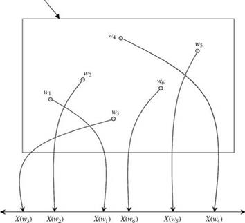
In analyzing the statistical features of infrastructural system responses, many events of interest can be defined by the related random variables. A random variable is a real-value function defined on the sample space. In other words, a random variable can be viewed as a mapping from the sample space to the real line, as shown in Fig. 2.4. The standard convention is to denote a random variable by an upper-case letter, whereas a lower-case letter is used to repre­sent the realization of the corresponding random variable. For example, one may use Q to represent flow magnitude, a random variable, whereas q is used to represent the values that Q takes. A random variable can be discrete or con­tinuous. Examples of discrete random variables encountered in hydrosystems infrastructural designs are the number of storm events occurring in a specified time period, the number of overtopping events per year for a levee system, and so on. On the other hand, examples of continuous random variables are flow rate, rainfall intensity, water-surface elevation, roughness factor, and pollution concentration, among others.

2.1.2 Cumulative distribution function

and probability density function

The cumulative distribution function (CDF), or simply distribution function (DF), of a random variable X is defined as

Подпись: (2.10)Fx (x) = P (X < x)

Random Variables and their Distributions

S

Random Variables and their Distributions

Figure 2.4 A random variable X(w) as mapped from the sample space to the real line.


The CDF Fx(x) is the nonexceedance probability, which is a nondecreasing function of the argument x, that is, Fx(a) < Fx(b), for a < b. As the argument x approaches the lower bounds of the random variable X, the value of Fx (x) approaches zero, that is, limx^-x Fx(x) = 0; on the other hand, the value of Fx(x) approaches unity as its argument approaches the upper bound of X, that is, limx^cx, Fx (x) = 1. With a < b, P (a < X < b) = Fx (b) – Fx (a).

For a discrete random variable X, the probability mass function (PMF), is defined as

Px (x) = P (X = x) (2.11)

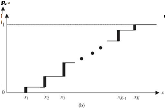
The PMF of any discrete random variable, according to axioms (1) and (2) in Sec. 2.1, must satisfy two conditions: (1) px(xk) > 0, for all xk’s, and (2) Sail kpx(xk) = 1. The PMF of a discrete random variable and its associated CDF are sketched schematically in Fig. 2.5. As can be seen, the CDF of a dis­crete random variable is a staircase function.

Подпись: fx(x) Random Variables and their Distributions Подпись: (2.12)

For a continuous random variable, the probability density function (PDF) fx( x) is defined as

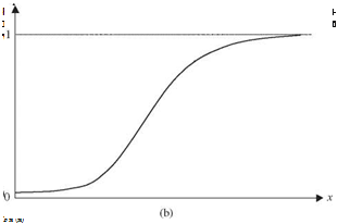
The PDF of a continuous random variable f x (x) is the slope of its corresponding CDF. Graphic representations of a PDF and a CDF are shown in Fig. 2.6. Similar to the discrete case, any PDF of a continuous random variable must satisfy two conditions: (1) fx(x) > 0 and (2) / fx(x) dx = 1. Given the PDF of a random variable X, its CDF can be obtained as

x

Подпись: (2.13)

Random Variables and their Distributions

fx(u) du

-TO

in which u is the dummy variable. It should be noted that fx ( ) is not a prob­ability; it only has meaning when it is integrated between two points. The probability of a continuous random variable taking on a particular value is zero, whereas this may not be the case for discrete random variables.

Random Variables and their Distributions

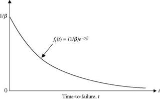
Example 2.6 The time to failure T of a pump in a water distribution system is a continuous random variable having the PDF of

ft(t) = exp(-t/1250)/e for t > 0, в > 0

in which t is the elapsed time (in hours) before the pump fails, and в is the parameter of the distribution function. Determine the constant в and the probability that the operating life of the pump is longer than 200 h.

Solution The shape of the PDF is shown in Fig. 2.7. If the function ft (t) is to serve as a PDF, it has to satisfy two conditions: (1) ft(t) > 0, for all t, and (2) the area under ft (t) must equal unity. The compliance of the condition (1) can be proved easily. The value of the constant в can be determined through condition (2) as

Random Variables and their Distributions Random Variables and their Distributions
Random Variables and their Distributions

1=


в


0


ft(t)

Random Variables and their Distributions

Figure 2.7 Exponential failure density curve.


Подпись: P(T > 200) = Random Variables and their Distributions Подпись: 200/1250 = 0 852

Therefore, the constant в = 1250 h/failure. This particular PDF is called the exponen­tial distribution (see Sec. 2.6.3). To determine the probability that the operational life of the pump would exceed 200 h, one calculates P (T > 200):

AFFORDABLE HOUSING – CHALLENGE AND RESPONSE

Подпись: IntroductionIn the nearly three decades since the national policy of "a decent home and a suitable living environment" was established in the Housing Act of 1949, millions of families have been able to reach the goal of home ownership. In recent years, however, this goal has proved elusive for others, particularly young families seeking to buy their first home.

Background,

The fundamental problem is that housing prices and mortgage interest rates rose faster than family incomes, particularly in the 1970’s. The median house price rose approximately 115 percent while incomes were increasing only about 105 percent. Even worse, during this period mortgage interest rates more than doubled, from below 9 percent to over 18 percent in many areas.

These figures are not precise, nor need they be to demonstrate the scope of the problem facing the nation in the early 1980’s. The fact is, many families were prevented from buying homes due to the increasing price of housing and cost of money.

Controlling mortgage interest rates is not something the housing industry can do independently; these rates reflect larger national economic issues. As a result of changes in the economic marketplace, by 1987 mortgage interest rates had dropped to about 10 percent, helping to make housing more affordable.

But housing prices have continued to rise; the median price of a house in 1986 was approximately 33 percent higher than it was in 1982. This increase was due to a number of factors, such as a trend to larger homes on larger lots, increasing amenities such as air conditioning and more bathrooms, higher material prices and labor costs, and sharply higher land costs around many of the nation’s major cities.

As will be seen in the ensuing chapters, the cost of land is often the largest single variable in the price of a house. Since land is a fixed quantity, the amount of land available for housing is constantly decreasing as new homes are built; utilizing land more efficiently is one of the best ways to make housing more affordable.

Studies by the President’s Commission on Housing in 1981, confirming earlier studies of the housing industry, also showed that excessive regulatory requirements and outmoded building practices also contribute to higher housing prices. In many instances, these studies pointed out that local officials and builders often were unaware of steps each could take to reduce housing costs.

The Joint Venture for Affordable Housing (JVAH) was initiated by Samuel R. Pierce, Jr., Secretary of Housing and Urban Development, in January 1982 to bring about changes in the way housing is controlled, designed, and built. Recognizing that many of these changes could only be made at the local level, Secretary Pierce organized the Joint Venture as a working partnership among the following organiza­tions and groups:

• American Planning Association

• Council of State Community Affairs Agencies

• International City Management Association

• National Association of Counties

• National Conference of State Legislators

• National Governors’ Association

• Urban Land Institute

• National Association of Home Builders (NAHB)

• NAHB National Research Center

• U. S. Department of Housing and Urban Development

BINDER DRAINDOWN TESTING

Various methods for testing the tendency for binder to draindown in a particular SMA are presented in Chapter 8. The original Schellenberg’s method and other techniques according to AASHTO and EN 12697-18 standards are also described there.

In most countries, Schellenberg’s or a similar method for determining the quantity of stabilizer in a mix has been applied. The maximum allowable mass of drained-off material is essentially the same almost everywhere and is equal to 0.3%. A recom­mended, safer limit is 0.2%.

4.2 SUMMARY

Factors influencing a mixture’s susceptibility to binder draindown are presented in Table 4.1.

TABLE 4.1

Summary of Factors influencing draindown potential in smA

effect on draindown potential

by decreasing

by increasing

Factor

Factor

Factor

Stabilizer content

Increase

Decrease

Stabilizer Type

Binder absorbers

Strong-to-medium decrease

Viscosity boosters

Medium-to-weak decrease (depending on type and temperature characteristics of used polymer)

sMA Mixture composition

Effective content of binder

Decrease

Increase

Content of sand fraction

Increase

Decrease

Content of filler

Increase

Decrease

components’ properties

Rigden voids (voids in a dry compacted filler)

Increase

Decrease

Aggregate absorption power (inversely Increase

Decrease

related to effective binder content)

Mixture production parameters

Production temperature

Decrease

Increase

Silo storage time of a hot mixture

Decrease

Increase

Note: SMA = stone mastic asphalt.

From the point of view of an SMA mix producer, stabilization efficiency is a decisive factor. But there is one more, equally important point: the quality of a stabi­lizer must be constant over the whole season of use. What does it matter, exactly, if a product is best at the moment of testing? If the quality varies, we may find ourselves wondering, “What happened? This cellulose is not as good as it used to be.” This variable quality often results in fat spots on the compacted SMA surface.

DEALING WITH SUPPLIERS AND SCHEDULING DELIVERIES

Estimating lumber and materials for a small, affordable house is fairly simple, but it does take some experience to get it right. If you are building a Habitat house, you can call or e-mail affiliates and ask them to share their lists with you (check the Habitat website for the affiliate in your area). You can also take a set of plans to a local supplier. Most building-supply outlets will create a materials list and give you a bid on what everything will cost. Always get bids from more than one supplier. Just make sure every supplier understands the type and grade of each item.

If you don’t make your own list, take the opportunity to in­spect the plans closely. Get acquainted with the house and all its parts before you start. Remember that a lumber list is only an estimate of materials that will be needed for a particular job. You may need to order a few more items as you build, or
you may need to send some materials back to the supplier. Find out ahead of time whether your suppliers charge a restocking fee for returned materials.

Most builders have materials delivered as needed, rather than all at once. You should do the same. That way, you won’t have to worry as much about storage problems. Also, ask your supplier to stack the lumber load in the order in which it will be used.

Some materials (especially trim, doors, and unpainted siding) should be stored indoors. When storing material out­side, set it on blocks above the ground and cover it with plas­tic to keep it dry. Be specific about where you want the lumber company to drop the wood, and pick a level, accessible loca­tion close to where it will be used. Hauling lumber by hand from any distance is hard, time-consuming work.

Подпись:DEALING WITH SUPPLIERS AND SCHEDULING DELIVERIESDEALING WITH SUPPLIERS AND SCHEDULING DELIVERIESПодпись: ItПодпись: —Подпись: (Подпись: 70]Подпись: /44 VMmПодпись: These hold-downs are attached to long bolts embedded in the concrete. They tie into the house frame and help keep a building on the foundation where it belongs. [Photo by Don Charles Blom] Подпись: Photo courtesy HFHIHabitat

for Humanity"

AN OPPORTUNITY FOR A NEW START

Salvador and Sara Arevalo almost decided not to partici­pate in the Jimmy Carter Work Project when it came to Los Angeles, CA, in 2007.

“We had another engagement," Salvador said, laughing. “But the affiliate urged us to attend."

During the event, the Arevalos (along with 29 other fami­lies) were given the opportunity to build a home for them­selves in just a matter of days. It was a family wish fulfilled.

Before their involvement with Habitat, the Arevalos never be­lieved they would own a home in Los Angeles. The high cost of housing in the city left them with few options.

Until recently they

occupied a one-bedroom fourplex, in urgent need of repair, with their three teenage daughters. Katy, soon to be a fresh­man in college, and Lesly, her youngest sister, slept in bunk beds in the dining room. Laria, 14, slept in a converted storage closet that she lovingly decorated.

When the opportunity arrived to work with Habitat, Salvador, who works in building maintenance, was eager to build his family’s home. Since the house’s completion, Salvador has dedicated himself to customizing and personal­izing the residence and making improvements when necessary.

“We are grateful to everyone who has made it possible for us to realize our dream of owning a house," he said.

Sara, who is quiet and reserved, was quick to answer when asked what advice she would give to someone considering a partnership with Habitat—“I would tell them not to miss the opportunity." —Heather Myers

к

MOISTURE CONTENT

Each day, a mature living tree can pump a ton of water into the atmosphere, so it’s no surprise that logs arrive at the mill with moisture contents of 30 percent to 55 percent. Consequently, a sawmill will rough-cut logs into lumber, air dry or kiln dry it, and then grade the lumber’s moisture con­tent before planing (surfacing) it.

Moisture content of 15 percent to 19 percent is optimal because that approximates the mois­ture content of ambient air in much of North America, except in the dry U. S. Southwest. Most often, lumber will be marked S-DRY or KD (kiln dried), indicating that its moisture content is 19 percent or less. KD-15 or MC-15 indicates a moisture content of 15 percent or less. Of course, even MC-15 lumber may be sopping wet if rained on during storage or transport. Wood that’s drier than MC-15 (say, 7 percent to 8 percent MC) may be a problem because it could swell after absorb­ing moisture on the job site—unless you live in the Southwest.

Подпись:Softwoods

Most construction lumber is called softwood, which is the lumber industry’s term for wood from conifers, the needle-leaved evergreens such as pine, fir, spruce, and hemlock. For the most part, these softwoods are softer and less dense than most hardwoods, which come from broad-leaved deciduous trees such as maple, oak, and walnut. That said, some softwoods, namely southern yellow pine, are much harder

A grade mark of S-GRN (surfaced green) indi­cates a moisture content more than 19 percent. Green lumber is hell to work with because it’s heavy (a green 8-ft.-long 2×4 can weigh 40 lb.), likely to distort, and certain to shrink—wreaking havoc with finish surfaces and trim. Thus S-GRN is a risky choice for renovations.

LUMBER SIZES

Lumber’s final size depends on milling processes. In smaller mills, lumber is often sawn, stickered, and allowed to air dry for 4 months to 6 months. If it’s not milled further, it’s called rough-cut lumber. Depending on the accuracy of the sawyer, the size may vary slightly, but the nominal size of, say, a rough-cut 2×4 is usually a full 2 in. by 4 in.

However, most lumber is rough cut and then surfaced (run through a planer to achieve uni­form thickness) before being kiln dried. At each stage, the lumber size decreases. Thus when you order a 2×4 (nominal size), you receive a piece with a 112-in. by 312-in. cross section (actualsize). Still, you pay for the nominal size.

Another way to size wood, especially hard­wood and Select finished woods, is by quarter – inch increments: 2/4, 3/4, 4/4, 5/4,6/4, and so on. The nominal actual difference is present here, too: For example, a nominal 5/4 stair tread is actually 1 in. thick.

PRESSURE-TREATED LUMBER

Lumber may also be marked as pressure treated. Such wood, after treatment, may be left exposed to weather, used near the foundation, or other­wise subjected to moisture, insects, or extremes of climate. If the wood will remain in contact with the soil, be sure that it is also rated for Ground Contact.

Since the 1940s, roughly 90 percent of all pressure-treated lumber was treated with CCA
(chromated copper arsenate). But the U. S. Environmental Protection Agency (EPA) deter­mined that CCA leaches arsenic into the soil; as a result, industry leaders agreed to stop using that treatment by the end of 2003. More benign types of pressure-treated lumber, such as.40 ACQ (alkaline copper quat) and CBA (copper boron azole) are available. Both biocides are arsenic free.

Whatever lumber treatment you consider, consult its product data sheets for the relative safety of the chemicals used and whatever care you should take when handling, storing, cutting, and applying it. In fact, it’s smart to capture and safely dispose of the sawdust.

ORDERING LUMBER AND CALCULATING BOARD FEET

The price of long thin pieces of wood, such as molding or furring strips, is based on their length, or lineal feet (lin. ft.). Sheet materials such as plywood and composite board are sold by the square foot, which is length times width; sheet thickness affects price, but it is not computed directly. Roofing and siding materials are often sold in squares of 100 sq. ft. Most yard lumber is sold by board feet, according to this formula:

width (in.) x thickness (in.) x length (ft.)

Подпись:12

Nominal and Actual Sizes of Softwood

NOMINAL

ACTUAL (in.)

1×2

3/4x1V2

1×4

3/4x3V2

1×6

3/4×51/2

1×8

3/4×71/4

1×10

3/4×91/4

1×12

3/4×111/4

2×4

11/2×31/2

2×6

11/2×51/2

2×8

11/2×71/2

2×10

11/2×91/2

2×12

11/2×111/2

Подпись: Seven Steps for On-Site Salvage If you are determined to do on-site salvage, here are a few suggestions: ► Get a tetanus shot and wear a long-sleeved shirt, heavy pants, thick-soled shoes, goggles, dust mask, gloves, and hard hat. ► Always cut power to the affected areas. Then use a voltage tester in outlets, fixtures, and switches to make sure there's no current flowing through them. ► Don't hurry. Look at the joints involved and remove the pieces slowly, bit by bit. ► As you free each piece, remove its nails immediately. Remember, footing on construction sites is chancy at best, and you don't want to land in a bed of nails when descending from a ladder in a hurry. ► If the piece is complex, such as a fireplace mantel, photograph it and then label the elements while carefully removing them. ► Before cutting salvage wood, scrutinize it closely for nails. Insert a pocket knife or an ice pick into suspect holes and check for hidden nails with a magnet. Then, still being concerned for hidden nails, use a carbide-tipped demolition sawblade and wear safety goggles. ► Most salvage is old, dry, and highly vulnerable to rot. Because it is dry, it will absorb moisture and rot before you know it. So get it under cover at once. In the two examples below, each board contains 1 board foot (bd. ft.):

12 in. x 1 in. x 1 ft.

= 1 bd. ft.

12

6 in. x 2 in. x 1 ft.

= 1 bd. ft.

12

In each of the following two examples, the dimensions given yield 2 bd. ft.:

12 in. x 1 in. x 2 ft.

= 2 bd. ft.

12

2 in. x 4 in. x 3 ft.

————————— = 2 bd. ft.

12

When calculating the total board feet of sever­al pieces of lumber, multiply the numerator (top part) of the fraction by the total number of pieces needed. Thus here’s how to calculate the board feet of 10 pieces of 2-in. by 6-in. by 12-ft. lumber:

2 in. x 6 in. x 12 ft. x 10

= 120 bd. ft.

12

Salvage Lumber

Salvage materials have striking advantages and disadvantages—the major plus being low cost; the major minus being prep time. Salvaging molding, flooring, and other materials from your own home is a good way to match existing mate­
rials, but be picky in selecting materials from other sources.

Reuse centers are popular these days. One example is Habitat for Humanity’s nonprofit stores, which offer tax deductions to donors and savings up to 75 percent off the original price of materials.

However, make sure all materials are struc­turally sound. Be sure to use a pocketknife to test lumber for rot or insects. Also treat with preser­vative any salvaged lumber that you’ll use as sills or that will be exposed to moisture.

Salvage materials usually aren’t worth the effort if they are in small quantities or if, after removing them, you find that they will be too short. Used 2x4s, for example, normally aren’t worth the trouble. By the time you yank them free from plates, remove nails, and cut off split ends, the studs may be only 7 ft. long.

Some materials just aren’t worth removing. For example, siding and other exterior trim is rarely worth saving, for it’s usually old and weather beaten. Barn board, in vogue years ago, is hardly charming when it is half-rotted, warped, and crawling with carpenter ants. If there is any danger of your destroying a piece of salvage by removing it, leave it alone. Parts of many beauti­ful old places that were restorable have been ruined by people who didn’t know what they were doing.

If you have any qualms about the structural strength of a building, stay out of it. Dismantling a building is a special skill, and inexperienced people who undertake the task can get hurt. Perhaps the best advice for would-be users of sal­vage materials is to buy it from a salvage yard. In this case, somebody has already done the dirty and dangerous work of removal.

Materials

Подпись: Dimension lumber is sawn from logs and then milled to a thickness and width that is slightly less than its nominal end cross sections. For example, the ends of these 2x6s actually measure 1 V> in. by Б1/ in.

This chapter of the

materials needed to frame and sheath a house. Materials include standard lumber; engineered lumber; sheet materials, such as plywood and particleboard; and fasteners, including nails, screws, and construction adhesives.

There’s never been a wider choice of building materials or more readily available information on using them, whether you need to size ceiling joists or find an environmentally safe adhesive that can bond frozen lumber. Just type your requirements into a Web site calculator or ask at your lumber supplier for a recommendation. Many related techniques are covered in Chapter 8.

Standard Lumber

Wood is a superb building material. It is strong, economical, and easily worked. Whether as a tree or as lumber, wood can withstand great loads, yet it’s resilient enough to regain its shape when loads are removed. Standard lumber is lumber sawn from logs in the traditional manner; where­as engineered lumber is often an amalgam of peeled, shredded, or reassembled wood pieces and strong adhesives.

LUMBER GRADES

After lumber has been milled, each piece is visu­ally graded according to established performance standards and then stamped. This grade stamp is important because building inspectors won’t approve structures built with unstamped lumber. Otherwise they’d have no way of knowing what loads the wood can support. In brief, grading is based on the presence of warping, knots, holes, decay, or other imperfections that could weaken the lumber and reduce its load-bearing capacity. Generally, dimension lumber grades are based on

Подпись:Подпись:Подпись:Подпись:Подпись:image112Подпись: PROnP Different species have different density, elasticity, and loadbearing capacity, so their lumber grades are not interchangeable. For example, a No. 1 HEM-FIR 2x10 may not have the same load/span capacity as a No. 1 southern pine 2x10. That's why structural engineers routinely specify both the grade and species of lumber (or species group) needed to satisfy requirements in building codes. llll strength, appearance, or both. The more imper­fections, the lower the grade.

Grade stamps indicate lumber grade, tree spe­cies, moisture content when the lumber was sur­faced, sawmill, and regional agency certifying the grading standards. Lumber that is stress rated by machine will have additional information.

Structural framing lumber grades run from Select Structural (the best looking and strongest) through No. 1, No. 2, and No. 3. An architect might specify Select Structural 4x8s, for exam­ple, when beams will be exposed in a living room. In most grading systems, No. 1 and No. 2 are

Here’s some standard lumberyard lingo:

► BOARDS are less than 2 in. thick and are used as trim, sheathing, subflooring, battens, doorstops, and such.

► LUMBER (dimension lumber) is 2 in. to 4 in. thick and is used for house framing: studs, posts, joists, beams, headers, rafters, stair carriages, and so on.

► FACTORY OR SHOP LUMBER is wood milled into window casings, trim, and other elements.

► TIMBER is at least 5 in. thick in its smallest dimension.

► STOCK applies to any building material in its unworked form, as it comes from the lumber­yard or mill.

► A STICK is jargon for a piece of lumber, such as a 2×4: "If that stick is too warped, go get another."

equally strong, though No. 1 has fewer cosmetic flaws. Thus if appearance is not a factor, you can order "No. 2 and better” without sacrificing strength. No. 3 is the weakest and least expensive grade in the structural category; you won’t save much by using it, because you’ll have to order larger dimensions to carry the same loads as No. 1 and No. 2 grades.

Light framing lumber, which is used for plates, sills, and blocking, has lower strength require­ments than structural framing members. Light framing members are 4 in. (thick or wide) or less. Grades are Construction (the best), Standard, and Utility. Contractors often order "Standard and better.”

Stud lumber is graded Stud or Economy Stud. In general, avoid Economy grade lumber of any kind. Although okay for temporary use, its inferior quality makes it unreliable in any sus­tained load-bearing situation.

LUMBER SPECIES

Species are denoted by abbreviations such as PP (ponderosa pine), DF (Douglas fir), and HEM (hemlock). Often, manufacturers will group species with similar properties. S-P-F (spruce, pine, fir) is by far the most common Canadian grouping, and HEM-FIR (hemlock-fir) is com­mon throughout the United States. Because lum­ber is heavy and expensive to ship, lumberyard sources tend to be from nearby mills. Since your lumberyard is likely to carry only a mixed stock of sizes and grades, your choice may be limited to what’s on hand.

Stabilizer Test Results

Almost every working road laboratory has conducted many series of draindown tests. The results of companion tests on a wide variety of stabilizers are seldom published. However, the following interesting conclusions can be drawn from large – scale research conducted in the United States (Brown and Mallick, 1994):

• SMA binder draindown was seen to be a time-progressive process; the fast­est run-off occurred within the first 30 minutes of hot mix storage, then it continued over 2 hours during testing. Therefore one can conclude that the major part of the draindown process takes place during the 1st hour after SMA production.

• The most effective stabilizers tested were cellulose and mineral fibers.

• Differences between binder-absorbing stabilizers and viscosity-enhancing stablizers were observed.

• Lack of a stabilizer caused as much as 4% (m/m) mastic drain-off in a 0/19 mm coarse-graded SMA.

During the course of a season of roadwork, we decide, for various reasons, to change the supplier of stabilizers, but we do not always have enough time to check the SMA draindown with the new product (after all, it looks more or less the same). At that time, we have to take into account some unexpected problems and be prepared to react quickly—for example, to increase the quantity of stabilizer, if needed.

JMF – Job Mix Formula – recipe of the mixture.

Total probability theorem and Bayes’ theorem

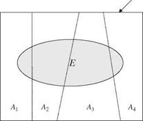
The probability of the occurrence of an event E, in general, cannot be deter­mined directly or easily. However, the event E may occur along with other attribute events Ak. Referring to Fig. 2.2, event E could occur jointly with K mutually exclusive (Aj П Ak — 0 for j — k) and collectively exhaustive (A1 U A2 U—U AK) — S attributes Ak, k — 1,2,…, K. Then the probability of the occur­rence of an event E, regardless of the attributes, can be computed as

KK

P(E) — P(E, Ak) — P (E | Ak)P(Ak) (2.8)

k—1 k—1

Equation (2.8) is called the total probability theorem.

Example 2.4 Referring to Fig. 2.3, two upstream storm sewer branches (I1 and I2) merge to a sewer main (I3). Assume that the flow-carrying capacities of the two up­stream sewer branches I1 and I2 are equal. However, hydrologic characteristics of the contributing drainage basins corresponding to I1 and I2 are somewhat differ­ent. Therefore, during a major storm event, the probabilities that sewers I1 and I2 will exceed their capacities (surcharge) are 0.5 and 0.4, respectively. For simplicity, assume that the occurrences of surcharge events in the two upstream sewer branches are independent of each other. If the flow capacity of the downstream sewer main I3 is

Total probability theorem and Bayes’ theorem

S


Figure 2.2 Schematic diagram of total probability theorem.


Total probability theorem and Bayes’ theorem

Figure 2.3 A system with three sewer sections.
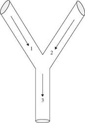
Total probability theorem and Bayes’ theoremthe same as its two upstream branches, what is the probability that the flow capacity of the sewer main I3 will be exceeded? Assume that when both upstream sewers are carrying less than their full capacities, the probability of downstream sewer main I3 exceeding its capacity is 0.2.

Solution Let E1, E2, and E3, respectively, be events that sewer I1, I2, and I3 exceed their respective flow capacity. From the problem statements, the following probabili­ties can be identified: P(E1) = 0.50, P(E2) = 0.40, and P(E3 | E1, E’2) = 0.2.

To determine P(E3), one first considers the basic events occurring in the two up­stream sewer branches that would result in surcharge in the downstream sewer main E3. There are four possible attribute events that can be defined from the flow con­ditions of the two upstream sewers leading to surcharge in the downstream sewer main. They are A1 = (E1, E2), A2 = (E1, E2), A3 = (E1, E2), and A4 = (E1, E2). Fur­thermore, the four events A1, A2, A3, and A4 are mutually exclusive.

Since the four attribute events A1, A2, A3, and A4 contribute to the occurrence of event E3, the probability of the occurrence of E3 can be calculated, according to Eq. (2.8), as

P(E3) = P(E3, A1) + P(E3, A2) + P(E3, A3) + P(E3, A4)

= P(E3 | A1)P(A1) + P(E3 | A2)P(A2) + P(E3 | A3)P(A3) + P(E3 | A4)P(A4)

To solve this equation, each of the probability terms on the right-hand side must be identified. First, the probability of the occurrence of A1, A2, A3, and A4 can be determined as the following:

P(A1) = P(E1, E2) = P(E1) x P(E2) = (0.5)(0.4) = 0.2

The reason that P (E1, E2) = P (E1) x P (E2) is due to the independence of events E1 and E2. Since E1 and E2 are independent events, then E1, E1, E2, and E2 are also

independent events. Therefore,

P(A2) = P(E, E2) = P() x P(E2) = (1 – 0.5)(0.4) = 0.2

P(A3) = P(E1, E2) = P(E1) x P(E2) = (0.5)(1 – 0.4) = 0.3

P(A4) = P(E1, E2) = P(E1) x P(E2) = (1 – 0.5)(1 – 0.4) = 0.3

The next step is to determine the values of the conditional probabilities, that is, P(E3 | A1), P(E3 | A2), P(E3 | A3), and P(E3 | A4). The value of P(E3 | A4) = P(E3 | E’, E2) = 0.2 is given by the problem statement. On the other hand, the values of the remaining three conditional probabilities can be determined from an understanding of the physical process. Note that from the problem statement the downstream sewer main has the same conveyance capacity as the two upstream sewers. Hence any up­stream sewer exceeding its flow-carrying capacity would result in surcharge in the downstream sewer main. Thus the remaining three conditional probabilities can be easily determined as

P(E3 | A1) = P(E3 | E1, E2) = 1.0 P(E3 | A2) = P(E3 | E1, E2) = 1.0 P(E3 | A3) = P(E3 | E1, E2) = 1.0

Putting all relevant information into the total probability formula given earlier, the probability that the downstream sewer main I3 would be surcharged in a major storm is

P(E3) = P(E3 | A1)P(A1) + P(E3 | A2)P(A2) + P(E3 | A3)P(A3) + P(E3 | A4)P(A4)

= (1.0)(0.2) + (1.0)(0.2) + (1.0)(0.3) + (0.2)(0.3)

= 0.76

Подпись: P (Ak | E) Подпись: P (Ak, E) P (E) Подпись: P (E | Ak) P (Ak) £^=1 P (E | Ak-) P (Ak') Подпись: for k = 1,2,..., K (2.9)

The total probability theorem describes the occurrence of an event E that may be affected by a number of attribute events Ak, k = 1, 2,…, K. In some situations, one knows P (E | Ak) and would like to determine the probability that a particular event Ak contributes to the occurrence of event E. In other words, one likes to find P(Ak | E). Based on the definition of the conditional probability (Eq. 2.6) and the total probability theorem (Eq. 2.8), P (Ak | E) can be computed as

Equation (2.9) is called Bayes’ theorem, and P (Ak) is the prior probability, rep­resenting the initial belief of the likelihood of occurrence of attribute event Ak. P (E | Ak) is the likelihood function, and P (Ak | E) is the posterior probability, representing the new evaluation of Ak being responsible in the light of the oc­currence of event E. Hence Bayes’ theorem can be used to update and revise the calculated probability as more information becomes available.

Example 2.5 Referring to Example 2.4, if surcharge is observed in the downstream storm sewer main I3, what is the probability that the incident is caused by simulta­neous surcharge of both upstream sewer branches?

Подпись: P(A1 | E3) Подпись: P(Ab E3) P (E3) Подпись: P (E3 | A1)P (A1) P (E3)

Solution From Example 2.4, A1 represents the event that both upstream storm sewer branches exceed their flow-carrying capacities. The problem is to find the conditional probability of A1, given that event E3 has occurred, that is, P(A1 | E3). This condi­tional probability can be expressed as

Подпись: P(A11 E3) Подпись: P (E3 | A1)P (A1) P (E3) Подпись: (1.0)(0.2) 0.76 Подпись: 0.263

From Example 2.4, the numerator and denominator of the preceding conditional prob­ability can be computed as

The original assessment of the probability is 20 percent that both upstream sewer branches would exceed their flow-carrying capacities. After an observation of down­stream surcharge from a new storm event, the probability of surcharge occurring in both upstream sewers is revised to 26.3 percent.