Airport in Frankfurt on the Main

One of the best-known applications of an SMA mixtures for airfields is the northern runway of the airport in Frankfurt on the Main (Fraport). It has become famous not only because of the SMA application but also because of the atypical arrange­ment of the reconstruction of the runway pavement. The 2-year long removal of the worn-out concrete pavement and the laying of a new asphalt structure was completed in 2005.

Fraport is one of the largest airports in the world, with a colossal traffic capac­ity and an impressive number of takeoffs and landings—more than 200,000 per year. The replacement of the northern runway pavement was carried out exclu­sively at night to reduce reconstruction-related air traffic problems. This necessi­tated organizational and technological arrangements to complete each stage of the reconstruction work early in the morning. The intended entrance to the work site was at 10:30 p. m. on a given night, followed by the first landing at 6:00 a. m. next day. The scope of work was divided into independent day lots (actually night lots), which had to be executed within a 7.5-hour break in takeoffs and landings.

The runway intended for rebuilding was 4000 m long and 60 m wide, for a total of 240,000 m2. The working lot reconstructed over one night was 15 m long. It took 300 nights to accomplish the pavement replacement. Work was started near the end of April 2003 and finished in June 2005. The old structure of the runway pave­ment comprised a set of cement concrete layers. All the new asphalt layers contained polymer modified bitumen (PmB) 25 or PmB 45, according to the German guide­lines for modified binders TL PmB 01. They were additionally supplemented with Fisher-Tropsch wax (Sasobit) to lower the compaction temperature of the asphalt. The Sasobit additive made possible the compaction of the asphalt mix at a lower tem­perature (usually at approximately 130°C) and faster cooling of the wearing course (the temperature after laying and compaction was about 100°C); this was critical since the mat had to cool within 1.5 hours prior to the first landing or takeoff at 6 a. m. The SMA 0/11 wearing course was 40 mm thick. Limestone with a hydrated lime additive was used as a filler. The SMA wearing course was spread at a speed of 5 m/min. Seven rollers were engaged in compacting the mat. At the moment of the first landing, the temperature of the pavement ranged between 52 and 79°C (Sasol GmbH, undated).

The replacement of Fraport’s northern runway pavement was successfully completed. At the same time it became one of the best-known runway reconstruction projects carried out without the disruption of transport services.

Subsurface Drainage System

Subsurface drainage is made up of different parts but all are linked directly with the surface drainage system and all are, fundamentally, taking care of groundwater or water that infiltrates through the pavement surface.

13.3.4.1 Drainage Regime

Part of the rainfall-runoff infiltrates into the ground and continues as subsurface flow. Part of this may, in turn, continue as a sub-horizontal subsurface flow, depend­ing on the permeability of different soil layers. This can lead to increases in the moisture level under the pavement, reducing the bearing capacity. To decrease this phenomenon, the scheme design should note that:

• it is a good practice in embankments in the Mediterranean countries either to keep the thickness between the underside of the pavement and the natural soil to at least 1.0 m, or, if necessary, a drainage layer (see below) as well as other measures should be used, depending of subsoil characteristics; and

• in a cutting, the depth of the lateral drains should allow for an adequate drainage depth to the groundwater level, normally more then 1.0 m.

Because of the different types of subgrade and pavement construction, it is important to be able to differentiate between those pavements where water flow will be largely vertical, wetting the subgrade (with the associated loss of subgrade support strength) and those situations where vertical water flow will be arrested by impermeable layers in the sequence, forcing the water sideways and necessitating different drainage measures. Figure 13.4 shows three types of pavements, A B and C, which are now described.

A. Subgrade layer with low permeability – infiltrated water will flow above the sub­grade, at the bottom of granular base/sub-base layers, according to the maximum crossfall;

B. Permeable subgrade layer and impermeable subsoil – infiltrated water flows on the layer between the subgrade and impermeable subsoil;

C. Permeable capping layer and subgrade – the water percolates vertically through every layer.

The basis for choosing whether approach Case A, B or C applies is set out in Fig. 13.5.

СЮ

Optimization techniques

Having constructed an optimization model, one must choose an optimization technique to solve the model. The way that one solves the problem depends largely on the form of the objective function and constraints, the nature and number of variables, the kind of computational facility available, and personal taste and experiences. Mays and Tung (1992) provide a rather detailed discus­sion on linear programming, dynamic programming, and nonlinear program­ming techniques. In this subsection, brief descriptions are given to provide
readers with some background about these techniques. A list of applications of various optimization techniques to hydrosystems engineering problems can be found elsewhere (Mays and Tung, 2005).

Linear programming (LP). LP has been applied extensively to optimal resource allocation problems. When the system under study is linear, LP models also can be used for parameter identification and system operation. By the name of the technique, an LP model has the basic characteristic that both the objective function and constraints are linear functions of the decision variables. The general form of an LP model can be expressed as

n

Подпись: Max (or min) subject toxo = ^ CjXj (8.3a)

j=i

n

‘^a. ijXj = bi i = 1,2,…, m (8.3b)

j=1

Xj > 0 j = 1, 2,…, n (8.3c)

where the Cj’s are the objective function coefficients, the aij’s are called the technological coefficients, and the bi’s are the right-hand-side (RHS) coefficients. An LP model can be expressed concisely in matrix form as

Max (or min)

xo = ctx

(8.4a)

subject to

Ax = b

(8.4b)

x > 0

(8.4c)

where c is an n x 1 column vector of objective function coefficients, x is an n x 1 column vector of decision variables, A is an m x n matrix of technological coeffi­cients, b is an m x 1 column vector of the RHS coefficients, and the superscript t represents the transpose of a matrix or vector. Excellent books on LP include Winston (1987), Taha (1987), and Hillier and Lieberman (1990).

The commonly used algorithm for solving an LP model is the simplex method developed by Dantzig (1963). Since its conception, the method has been used widely and considered as the most efficient approach for solving LP problems. The simplex algorithm, starting at an initial feasible solution to the LP model, searches along the boundary of a problem’s feasible space to reach the opti­mal solution. The method has been applied to solve large problems involving thousands of decision variables and constraints on today’s computers. Com­puter codes based on the simplex method are widely available. Some of the well-known LP software includes GAMS (general algebraic modeling system) by Brooke et al. (1988) and LINDO (linear, interactive, and discrete optimizer) by Schrage (1986), for which PC versions of the programs are available. For LP
models, because of the convexity of the feasible region, the solution obtained is a global optimum.

Two additional methods for solving LP problems have been developed that apply different algorithmic strategies (Khatchian, 1979; Karmarkar, 1984). In contrast to the simplex algorithm, Khatchian’s ellipsoid method and Karmarkar’s projective scaling method seek the optimum solution to an LP problem by moving through the interior of the feasible region.

Nonlinear programming (NLP). A nonlinear programming model has the general format of Eqs. (8.1a-c) in which either the objective function f (x) or the con­straints g (x) or both are nonlinear. In an NLP problem, the convexity of the feasible space defined by the nonlinear constraints g (x) is generally difficult to assess. As a result, the solution obtained by any NLP algorithm cannot guar­antee to be globally optimal. Detailed description for solving NLP problems can be found in Edgar and Himmelblau (1988), Fletcher (1980), McCormick (1983), and Gill et al. (1981).

Basically, algorithms for solving NLP problems are divided into two cate­gories: unconstrained and constrained algorithms. Unconstrained NLP algo­rithms solve Eq. (8.1a) without considering the presence of constraints. They provide the building blocks for the more sophisticated constrained NLP algo­rithms. Consider an unconstrained NLP problem

Minimize f (x) x є Kn (8.5)

in which Kn is an n-dimensional real space. Assume that f (x) is twice dif­ferentiable; the necessary conditions for x* to be a solution to Eq. (8.5) are (1) Vxf (x*) = 0 and (2) V| f (x*) = H(x*) is semipositive definite in which Vxf = (d f /д x1, d f /д x2,…, d f /dxn)t, agradient vector of the objective function and Vx2 f = (д2 f /дxiдxj) is an nx nHessian matrix. The sufficient conditions for an unconstrained minimum x * are (1) Vxf (x *) = 0 and (2) Vxf (x *) = H (x *) is strictly positive definite.

In theory, the solution to Eq. (8.5) can be obtained by solving Vxf (x*) = 0, which involves a system of n nonlinear equations with n unknowns. This ap­proach has been regarded as indirect because it backs away from solving the original problem of minimizing f (x). Furthermore, numerical iterative proce­dures are required to solve the system of nonlinear equations which tend to be computationally inefficient. Therefore, the general preference is given to those solution procedures which directly attack the problem of optimizing the objec­tive function. Like the LP solution procedure, direct solution methods, during the course of iteration, generate a sequence of points in the solution space that converge to the solution of the problem by the following recursive equation:

x(r+1) = x(r} + в(r}d(r} r = 1,2,… (8.6)

in which the superscript (r) represents the iteration number, x is the vector of the solution point, d is the vector of the search direction along which the objective function f (x) is to be minimized, and в is a scalar, called the step size, that minimizes f (x(r) + в(r)d(r)). This procedure is called the line search or one-dimensional search. Several unconstrained NLP algorithms have been developed, and they differ by the way the search directions are determined during the course of iteration. Mays and Tung (1992, p. 136) summarize the search directions of various methods.

Without losing generality, consider a nonlinear constrained problem stated by Eq. (8.1) with no bounding constraints. Note that the constraints Eq. (8.1b) are all equality constraints. Under this condition, the Lagrangian multiplier method can be applied, which converts a constrained NLP problem to an uncon – strainted one by an augmented objective function called the Lagragian. That is, Eqs. (8.1a-b) can be written as

Minimize L(x, X) = f (x) + Xіg(x) (8.7)

in which L(x, X) is the Lagrangian function, X is the vector of m Lagragian multipliers, and g(x) is the vector of constraint equations. The new objective function L(x, X) involves n + m decision variables. The necessary condition and sufficient conditions for x* to be the solution for Eq. (8.7) are

1. f (x*) is convex, and g(x*) is convex in the vicinity of x*.

2. VXL(x*, X) = 0.

3. VxL(x*, X) = g(x*) = 0.

4. X’s are unrestricted in sign.

Solving conditions 2 and 3 simultaneously yields the optimal solution to Eq. (8.7).

The most important theoretical results for the NLP problem are the Kuhn – Tucker conditions, which can be derived easily by using the Lagrangian method for the general NLP problem, as stated in Eq. (8.1a-c). These conditions must be satisfied at any constrained optimum, local or global, of any LP or NLP problem. They form the basis for the development of many computational algorithms.

Several NLP computer codes are available commercially. They are the GRG2 (generalized reduced gradient 2) developed by Lasdon and his colleagues (Lasdon et al., 1978; Lasdon and Waren, 1978); (2) GINO (Liebman et al., 1986); (3) MINOS (modular in-core nonlinear optimization system) by Mautaugh and Saunders (1980, 1983), and (4) GAMS-MINOS, a link for GAMS and MINOS. Microsoft Excel SOLVER implements GINO in a spreadsheet working environment.

Dynamic programming (DP). Before performing the optimization, it is sometimes desirable to make some changes of variables and transformations so that the model can be solved more efficiently. However, one must keep in mind that such transformations should completely preserve the properties of the original problem (model) so that the transformed model will yield the optimal solution to the original problem. Basically, DP is such a transformation that takes a sequential or multistage decision process containing many interrelated decision variables and converts it into a series of single-stage problems, each containing only one or a few variables. In other words, the DP technique decomposes an n-decision problem into a sequence of n separate but interrelated single-decision subproblems. Books that deal with DP are Dreyfus and Law (1977), Cooper and Cooper (1981), and Denardo (1982).

To describe the general philosophy of the DP technique, consider the fol­lowing resource allocation problem (Tung and Mays, 1992). Suppose that one wishes to allocate funds to three water development projects, A, B, and C, to maximize the total revenue. Each development project consists of several alter­native configurations that require different funding levels and yield different revenues. Owing to the budget limitation, the total available funds for the en­tire development are fixed. If the number of alternatives for each project is not too large, one probably can afford to enumerate all possible combinations of project alternatives exhaustively to identify the optimal alternatives for the entire project development. This brute-force exhaustive enumeration approach possesses three main shortcomings: (1) It would become impractical if the num­ber of alternative combinations is large, (2) the optimal course of action cannot be verified, even it is obtained in the early computations, until all the combi­nations are examined, and (3) infeasible combinations (or solutions) cannot be eliminated in advance.

Using the DP technique, one considers the selection of alternatives within each project individually without ignoring the interdependence among the projects through the total available budget. Since the total funds are limited, the amount available to each project depends on the allocations to the other projects. Whatever funds are given to project A and project B, the allocation to the remaining project C must be made to optimize its return with respect to the remaining capital. In other words, the optimal allocation to project C is condi­tioned only on the available funds for project C after allocations to project A and project B are made. Since one does not know the optimal allocations to project A and project B, the optimal allocation and the corresponding revenue from project C must be determined for all possible remaining funds after allocations to project A and project B have been made. Furthermore, whatever amount is allocated to project A, the allocations to project B and project C must be made optimal with respect to the remaining funds after the allocation is made to project A. To find the optimal allocation to project B, one finds the allocation maximizing the revenue from project B together with the optimal revenue from project C as a function of remaining funds from the allocation to project B. Finally, the optimal allocation to project A is determined, to maximize the rev­enue from project A plus the optimal revenue from both project B and project C, as a function of the funds remaining after the allocation to project A.

This description of the DP algorithm applied to a budget allocation example can be depicted schematically as Fig. 8.3, from which the basic elements and terminologies of a DP formulation are defined.

Return Return Return

from A from B from C

Optimization techniques

Decision Decision Decision

for A for B for C

Figure 8.3 Dynamic programming diagram for budget allocation example.

1. Stages (n) are the points in the problem where decisions are to be made. In the funds allocation example, each different project represents different stages in the DP model.

2. Decision variables (dn) are courses of action to be taken for each stage. The decision in each stage (project) is the alternative within the project to be selected for funding. The number of decision variables dn in each stage is not necessarily equal to one.

3. State variables (Sn) are variables describing the state of a system at differ­ent stages. A state variable can be discrete or continuous, finite or infinite. Referring to Fig. 8.3, at any stage n, there are the input state Sn and the output state Sn+1. The state variables of the system in a DP model have the function of linking between succeeding stages so that when each stage is optimized separately, the resulting decision is automatically feasible for the entire problem. Furthermore, it allows one to make optimal decisions for the remaining stages without having to check the effect of future decisions on the decisions made previously. Given the current state, an optimal policy for the remaining stages is independent of the policy adopted in the previous stages. This is called Bellman’s principle of optimality, which serves as the backbone of the optimization algorithm of the DP technique.

4. Stage return (rn) is a scalar measure of effectiveness of the decision made in each stage. It is a function of input state, output state, and the decision variable of a particular stage. That is, rn = r (Sn, Sn+1, dn).

5. State transition function (t„) is a single-valued transformation that expresses the relationships between input state, output state, and decision. In general, through the stage transition function, the output state Sn+1 at any stage n can be expressed as the function of input state Sn and the decision dn as

Sn+1 = tn(Sn, dn) (8.8)

The solution begins with finding the optimal decision for each possible state in the last stage (called the backward recursive) or in the first stage (called the forward recursive). Usually, one can exchange the sequence of the decision-making process. Hence which end to begin will be trivial. A recursive relationship that identifies the optimal policy for each state at any stage n can be developed, given the optimal policy for each state at the next stage n + 1. This backward-recursive equation, referring to Fig. 8.4, can be written as

f*(Sn) = optdn{rn(Sn, dn)} for n = N

= optdn {r n( Sn, dn) о f*+1[tn( Sn, dn)]} for n = 1,2,…, N – 1 (8.9)

in which о represents a general algebraic operator that can be +, -, x, or others.

The efficiency of an optimization algorithm is commonly measured by the computer time and storage required in problem solving. In the DP algorithm, the execution time mainly arises from the evaluation of the recursive formula, whereas the storage is primarily for storing the optimal partial return and the decision for each feasible state in each stage. DP possesses several advantages in solving problems involving the analysis of multiperiod processes; however, there are two major disadvantages of applying DP to many hydrosystems prob­lems, i. e., the computer memory and time requirements. These disadvantages would become especially severe under two situations: (1) when the number of state variables is beyond three or four and (2) when DP is applied in a discrete fashion to a continuous state space. The problem associated with the second situation is that difficulties exist in obtaining the true optimal solution without having to considerably increase discretization of the state space.

Because of the prohibitive memory requirement of DP for multidimensional systems, several attempts have been made to reduce this problem. One such modification is the discrete differential DP (DDDP). The DDDP is an iterative DP that is specially designed to overcome the shortcomings of the DP approach. The DDDP uses the same recursive equation as the DP to search for an improved trajectory among discrete states in the stage-state domain in the vicinity of an initially specified or trail trajectory (Heidari et al., 1971). Instead of searching over the entire state-stage domain for the optimal trajectory, as is the case for DP, DDDP examines only a portion of the state-stage domain, saving a considerable amount of computer time and memory (Chow et al., 1975). This optimization procedure is solved through iterations oftrial states and decisions to search for optimal returns (maximum or minimum) for a system subject to the constraints that the trial states and decisions should be within the respective admissible domain in the state and decision spaces.

ri

f

Г2 1

Гп

Гn+1 1

rN

Stage

1

Stage

1

__ ^ …. _Sn^

Stage

n

Sn+1 —►

Stage n + 1

__ ^ ___ Sn ^

Stage

N

1

d1

1

d2

dn

1

dn+1

dN

Figure 8.4 Schematic diagram of dynamic programming representation.

General purpose computer codes for solving DP problems are not available commercially because most problems are very specific and cannot be cast into a general framework such as Eqs. (8.1a-c). Therefore, analysts often have to develop a customized compute code for a specific problem under consideration.

Global optimization techniques. To optimize a complex hydrosystem involving a large number of interrelated decision variables, it is generally difficult to be certain that the optimal solution can be obtained within a reasonable amount of time. In dealing with such “hard” problems, one could opt to obtain the optimal solution with the anticipation to consume a vary large amount of computational time using the optimization techniques previously mentioned or to reach a quick but good solution that is suboptimal through some approximate or heuristic al­gorithms. Simulated annealing (SA) and genetic algorithm (GA) are two types of high-quality general algorithms that are independent of the nature of the problem. Both SA and GA, by nature, are randomization algorithms that apply a local search based on stepwise improvement of the objective function through exploring the neighboring domain of the current solution. The quality of the local optimum can be strongly dependent on the initial solution, and in prac­tice, it is difficult to assess the time needed to reach the global optimum. To avoid being trapped in a local optimum, local search algorithms can (1) try a large number of initial solutions, (2) introduce a more complex neighborhood structure to search a larger part of the solution space, and (3) accept limited transitions to explore the solution space in which the solution is inferior (Aarts and Korst, 1989).

Simulated annealing algorithms. The simulated annealing (SA) algorithms solve optimization problems by using an analogy to physical annealing process of decreasing temperature to lower energy in a solid to a minimum level. The annealing process involves two steps: (1) increasing the temperature of a heat bath to a maximum value at which the solid melts, and (2) decrease carefully the temperature of the heat bath to allow particles to arrange themselves in a more structured lattice to achieve minimum energy level. If the temperature of the heat bath decreases too rapidly (called quenching), the solid could be frozen into a metastable state in which the solid would be brittle. The connection between optimization and the annealing process was first noted by Pincus (1970) and formalized as an optimization technique by Kirkpatrick et al. (1983).

SA algorithms employ random search, which not only accepts solutions that improve the current solution but also accept solutions that are inferior with a specified probability according to the Metropolis criterion, that is,

Optimization techniques

(8.10)


where x-1 is the optimal solution in the r th iteration, x j +1 is the j th trial solution of the (r + 1)th iteration, f ( ) is the objective function value analogous
to the energy level of a solid, and T is the control parameter analogous to the temperature of the heat bath. As can be seen from Eq. (8.10), in a subsequent iteration a new trial solution yielding an objective function value that is a worse objective function value compared with the current optimum one will have lower (but not zero) probability of being accepted than a solution producing a better objective function value.

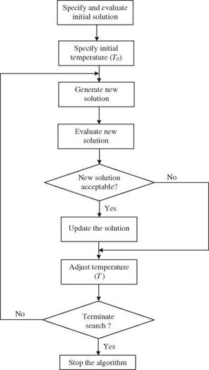
Implementation of the SA algorithm is remarkably easy, as shown in Fig. 8.5, which involves the following steps: (1) generation of possible solutions to explore

Optimization techniques

Figure 8.5 Algorithm of simulated annealing.

the solution space, (2) evaluation of the objective function, and (3) definition of the annealing schedule specified by the initial control parameter T0, decrement of control parameter AT, and convergence criteria. Mechanisms for generat­ing trial solutions in each iteration involve introducing random changes with the intent to cover the solution domain to be searched. The domain of search generally changes with the iteration, and there are many ways to implement domain search (Vanderbilt and Louie, 1984; Parks, 1990).

Since SA algorithms only require objective function evaluation at each gener­ated trial solution, computational efficiency of the entire process could become an important issue because implementation of the algorithms anticipates a large number of function evaluations. Many optimization problems in hydrosys­tems engineering involve objective functions whose values depend on physical constraints defined by complex flow simulations. In such cases, it is worthy of the effort to search and implement more computationally efficient procedures. To handle constraints in an SA algorithm, the simplest way is to reject the trial solution if it leads to a constraint violation. Alternatively, penalty function can be introduced to account for the constraint violations.

In implementation of the SA algorithm, T0 is generally set to be high enough to allow virtually all trial solutions to be accepted. It is analogous to having the temperature in the heat bath high enough to “melt” the solid. It is equivalent to the acceptance probability for T0 being close to 1. As the solution improves with the iterations, the control parameter T gradually decreases in value. The SA iteration is terminated when the control parameter T reaches a specified final value or the total number of trial solutions is reached. Alternatively, one can halt the algorithm if lack of improvement in the objective a function value is defined, which can be (1) no improvement can be found in all trial solutions at one control parameter and (2) acceptance ratio falls below a specified value.

Genetic algorithms. Genetic algorithms (GAs) are a class of computer-based search procedures that emulate the biologic evolution processes of natural se­lection and genetics. Since its introduction by Goldberg in 1983, this innovative search procedure has been applied widely for optimization in a wide variety of areas (Goldberg, 1989). GAs have been demonstrated to be robust search proce­dures that outperform the conventional optimization procedures, in particular for problems with high dimensionality, discontinuities, and noise.

Using GA for optimization, analogues are made between the properties of an optimization problem and the biologic process of gene selection and reproduc­tion. The solution space for an optimization problem can be treated as the en­vironment in which potential solutions can be considered as genes. The degree of fitness of each gene can be measured by the value of the objective function of an optimization problem. In each iteration of a GA search, several genes rep­resenting solutions are generated from the population. These genes compete for their survival based on their fitness: The one that is fitter is more likely to survive and influence the next generation. Through this competition, the pop­ulation evolves to contain high-performance individuals. In a GA, iteration is represented by a generation, and decision variables are analogous to biologic genes and are represented by coded structures either in the form of a real num­ber or binary codes. A point in the solution space is represented by a collection of genes, and the coded genes are juxtaposed to form an individual or chromosome.

Like any optimum-seeking algorithm, a GA requires the specification of an initial population (the first generation) of potential solutions. This can be done by random generation of a population or by specifying an initial solution. In the initial population, the fitness of an individual is evaluated with respect to the objective function. Those individuals with a high level of fitness will have higher chance being selected to produce offspring than those individuals with a lower level of fitness. The selection can be conducted in many different ways, such as stochastic universal sampling (Baker, 1987), which behaves like a roulette wheel with the slot size apportioned to each individual’s relative fit­ness in the population. The principle of the selection is to prefer better solutions to worse ones. This very feature of the selection procedure in a GA is similar to the Metropolis acceptance criterion of SA algorithms. The implementation of such selection procedure will prevent the solutions from being trapped at the local optimum.

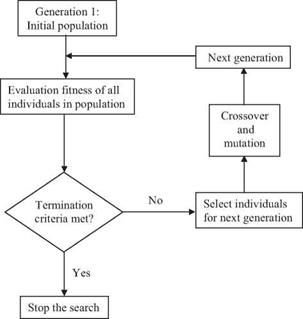
On the completion of selection of individuals in a generation, individuals selected will mate to produce the population of the next generation. During the mating, biologic processes of gene crossover and mutation could take place. Again, fitness of individuals in the population of the new generation will be evaluated based on which selection and mating processes will be repeated. A schematic diagram of a GA is shown in Fig. 8.6. Through this repeated

Optimization techniques

Figure 8.6 Schematic diagram of genetic algorithm.

fitness-selection-reproduction cycle, the population generated by the GA will evolve toward improved solutions.

Two main mechanisms are involved for those selected individuals to generate offspring in the next generation, i. e., crossover and mutation. Crossover allows information exchange between two chosen individuals forming the parents. In GA, crossover is done by randomly selecting positions in a chromosome of two individuals to swap their coded genes to produce the offspring. The rate of crossover has been suggested to be from 0.6 to 1.0 (Goldberg, 1989). Mutation then is a process by which new genetic materials can be introduced into the population. It is applied on a bit-by-bit basis, with the mutation rate specified by the user.

STEP2 Install the Interior Doors

Once the underlayment is down, start installing the prehung doors. I have lived in older houses that required work on sticky doors, misaligned locks, and squeaky hinges. Quality doors open and close with ease even after years of use—if you take the time to install them with care. Remember that doors and jambs should last for the life of the house. That won’t happen if you buy junk. Doors and trim are finish work and are seen and used on a daily basis, so try to buy units that are both attractive and durable (see the side – bar on p. 244).

The first step in setting prehung doors is lo check the plans and see which way they open into a room. It’s helpful to set each door near its opening before nailing any of them in place. This should eliminate installing the wrong door in an opening. Whichever style

of prehung door you have, the installation process is basically the same. If the floors will be carpeted, put а Уь-іп.-thick block of OSB or plywood (V in. wide by 1 in. long) under each jamb side. The block will be hidden once the floor is carpeted. Otherwise, unless you have ordered shortened doors, you may have to trim the bottom of the door so it won’t drag on the carpet. The block, especially important when setting a heavy door, keeps the door assembly from settling, causing the door to stick.

Professional trim carpenters often order shortened doors from the supplier. That allows them to set the jambs right on the sub­floor without having to raise them for carpet­ing. There is no need to buy shortened doors for thin vinyl floors. Check to see what other builders are doing in your area.

If a door is to work properly, its jamb needs to be set plumb, square, straight, and cross-sighted (both side jambs parallel to, or

Подпись:
STEP2 Install the Interior DoorsПодпись: PREHUNG DOORS ARE EASY TO INSTALL. Drive the first nail through the jamb and into the trim-mer, near the top on the hinge side.STEP2 Install the Interior DoorsSTEP2 Install the Interior Doors

THE STANDARD INTERIOR DOOR used in most affordable homes is 32 in. wide and has a flat, smooth plywood "skin" that covers a hollow core. But instead of settling for standard hollow-core doors, I recommend shopping around for some frame-and-panel doors made from solid wood. Doors can be a source of beauty in your house, and it may

be worth the extra cost to have some well-crafted doors in your favorite door­ways. Check with one or more local suppliers, and look at the array of doors that are available. Some­times, styles are discontin­ued or doors are special – ordered but never claimed. When that happens, you can find a great door at a bargain price.

Most doors open into rooms rather than into a hallway. They seldom open into closets. They can swing either to the right or to the left. The swing,

or hand, of a door can be confusing (see p. 157).

Make sure when you order doors that you and your supplier are both on the same page. Most house plans show which way the doors swing, so it’s not a bad idea to take the plans with you when you order doors.

Different styles of pre­hung doors are used in dif­ferent parts of the country.

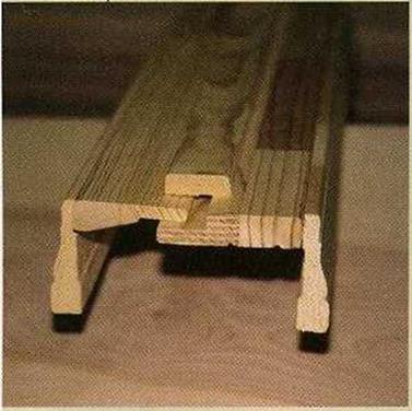
I like split-jamb, prehung doors, because they come with the trim (casing) installed, and they adjust for uneven wall thicknesses (see the photo at left). Another type of prehung door has a knockdown jamb. It comes in three pieces and also has the cas­ing installed. A third style of prehung door has just the jambs but no casing (see the photo above).

After the jambs have been nailed in place, the cas­ing must be cut and nailed around them.

in plane with, each other), so pay attention to the steps in the sidebar on the facing page. Remove any nails or plugs installed at the fac­tory to hold the jamb and door together. Set the prehung assembly in the opening, and drive a 6d or an 8d finish nail through the jamb, about 3 in. or so from the top on the hinge side (see the photo at left).

With any luck, the trimmer on the hinge side will be plumb and you can nail the jamb directly to it without the use of shims. Use a 4-ft. level to check the hinge-side jamb for plumb and straight. Make sure the margin between the underside of the head jamb and the top of the door is at least % in., about the

And Crown Molding

As noted in "The Case for Not Leveling Trim,” on p. 415, baseboard and crown molding should follow floors and ceilings, rather than level lines projected across the walls. If floors and ceilings are level, fine. Otherwise, leveled trim next to out-of-level surfaces is glaringly obvious.

INSTALLING BASEBOARDS

Install the finish floors first, with a slight gap, typically i<2 in., between the wood flooring and the walls so that wood strips or planks can expand and contract seasonally. Baseboards thus cover that gap along the base of the walls. You should also install door casing before baseboards, so that baseboards can butt to side casing or plinth blocks. Back-cutting the baseboard slightly yields a tight butt joint against plinth blocks or casing, even if the trim boards are not perfectly square to each other.

Locating studs beforehand will make installa­tion easier. If walls have been newly drywalled, look along the base of the walls for screws or nails where panels are secured to stud centers. Otherwise, rap the base of walls with your knuckle till you think you’ve found a stud. Then drive in a 6d finish nail to locate the stud exactly. Stud – finders work, but they are less reliable with plaster walls, whose lath nails meander all over the place.

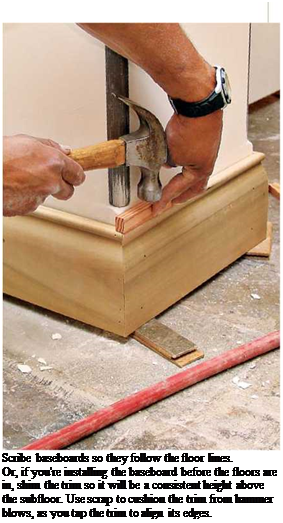
Scribe the bottom of baseboards to follow the contour of the floor, especially if the floors are irregular. But first, shim the baseboard(s) up about 1 in. above the floor, butt one end of the board to a corner or a door casing, and tack the baseboard to a stud or two to keep it upright. Then run the scribe or compass along the bottom to transfer the floor contour to the baseboard.

Cut the scribed line with a fairly rigid jigsaw blade that can cut with the grain; a Bosch T1001D™, with 6 TPI works like a charm.

Baseboard joinery employs basic techniques described earlier. Miter outside corners, cope inside ones, and glue all joints before nailing

image878
CASING AN ARCHED WINDOW

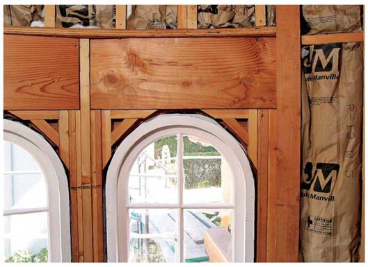
Arched windows require complex framing around the arch so you have something solid to nail finish walls and casing to.

image879

Подпись: 2. After cutting the arched casing at its spring lines, align the inner edge of the arched casing to the reveal line.

1. After scribing a reveal line along the edge of the arched head jamb, tack a finish nail at the apex of the line, and hang (balance) the arched head casing from it. Then level across the "spring lines" of the casing—the points at which the casing springs into its curve.

4. Work around the window, nailing the casing every 16 in. The thickness of the casing determines the nail size. In this case, the carpenter used 1-in. brads to nail the inside edge of casing to the frame edges, and 6d finish nails along the outside.


3. Next, install the straight side casing, cutting it a little long on the bottom and then trimming as needed till the casing fits tightly between the arched head casing and the window stool. After dry-fitting the side casing, apply glue, and tack it up.


5. If the casing is not wide or thick enough for biscuit joinery, angle 6d finish nails to draw the joint together. To avoid splitting the casing, you first need to snip off the nail points.


image881image882image883

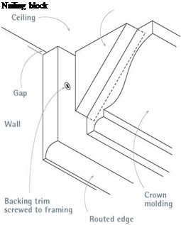
Подпись: I Crown Molding and Blocking
Подпись: Nailing block

Подпись: Scribe baseboards so they follow the floor lines. Or, if you're installing the baseboard before the floors are in, shim the trim so it will be a consistent height above the subfloor. Use scrap to cushion the trim from hammer blows, as you tap the trim to align its edges. When installing nailing blocks without backing trim, nail the blocks directly to the wall plates. Keep a 1/16-in. space between the back of the molding and the face of the blocks to accommodate wall-ceiling irregularities.

Подпись: PROnP When ripping down a baseboard, keep the sawblade just off the scribed pencil line. After cutting, clamp the board to a bench and sand exactly to the line, using a belt sander held perpendicular to the board edge. In this case, 80-grit to 120-grit sandpaper is effective because it's not overly aggressive. 1111

them off. Use two 8d nails (aligned vertically) at every other stud center, and use a single 4d finish nail top and bottom to draw mitered corners tight. Used as baseboard caps, standard mold­ings, such as quarter-rounds, can hide irregulari­ties between the top of the baseboard and the wall, and they dress up the top of the board. Where baseboards abut door casing and there’s no stud directly behind the end of the baseboard, nail the bottom of the board to the wall plate, and angle-nail the top to the side of the casing or plinth block, using an 18-gauge brad to avoid splitting the trim. Finally, set the nails, fill the holes, and caulk all seams before painting.

Pros and Cons of SMA for Airfields

Despite the fast growth of applications on road pavements, SMA does not enjoy great success on airfields. This is because of the unique requirements for airfield pave­ments and special problems with SMA, which include the following:

• Combining high macrotexture with low permeability

• Low-initial antiskid properties and the impossibility of using gritting (FOD risk)

• Risk of segregation (e. g., fat spots, porosity) locally changing the surface properties

Regardless of the cited weak points of SMA, airport managers sometimes decide to apply it, taking into consideration the strong points known from the road industry. A comprehensive survey of SMA applications on airports may be found in Prowell et. al. (2009).

WHEN ГМ FEELING NOSTALGIC, I think about the fancy, vvell-crafted toolkit I carried

from job to job before 1 switched to a 5-gal. plastic bucket. That kit had a place for all my finish tools—handsaws, levels, small hammers, razor-sharp chisels with their blades wrapped in soft cotton, and planes that left long curls of wood with each pass. My brother, Jim, still has his shiny, metal miter box with its long backsaw—that’s what we used to make perfect cuts in trim before chopsaws came along. Back in the late 40s and early ’50s, those were the tools that master builders passed down to us “kids" as they taught us the craft.

Today, carpentry is different. Power tools dominate—from motorized miter saws (chopsaws) and pneumatic nailers to cordless drills, belt sanders, random-orbit sanders, and jigsaws. And many of the things we used to build at the job site, such as kitchen cabinets, bathroom vanities, and door and window jambs, are now factory – made products that arrive ready to install. Despite these changes, basic hand-tool and careful layout skills are still essential, especially at this stage of the game, when the rough frame of the house, with all its imperfections, has been covered by drywall, and the walls have been painted. Now it’s time to prepare floors for vinyl and carpet;

Подпись: STEP BY STEPПодпись: 1 2 3 4

Install Underlayment for Vinyl Flooring Install the Interior Doors Install the Window and Door Casings Install the Cabinets

5 Install the Countertops

6 Install the Baseboard and Chair Rail

7 Trim Out the Closets

Interior Trim, Cabinets, Countertops, and Clost

Interior Trim, Cabinets, Countertops, and Clost

install interior doors, window casing, and interior trim; and secure cabinets and counter – tops. Do this work right, and the inside of your house will begin to look beautiful and much more livable.

STEP 1 Install Underlayment for Vinyl Flooring

Because vinyl flooring is quite thin, it is com­mon to install sheets of underlayment over a subfloor to provide a smooth, level base for the vinyl. Typically just M in. thick, 4×8 under­layment sheets can be made of particleboard (wood particles glued together under pres­sure), MDF (medium-density fiberboard, a smoother version of particleboard), or ply­wood. Ї like to install underlayment in the kitchen and bathroom after the drywall is fin­ished but before the cabinets or prehung doors are installed.

Underlayment must be installed on a rela­tively clean floor. Remove all globs of joint compound from the subfloor throughout the house and give it a good vacuuming. I prefer vacuuming (with a rugged, wet-dry vac, not a home model) to sweeping, because sweeping can create a dust storm. Some builders apply beads of construction adhesive before install­ing underlayment. A clean floor allows you to do this. Adhesive won’t adhere to a dirty floor.

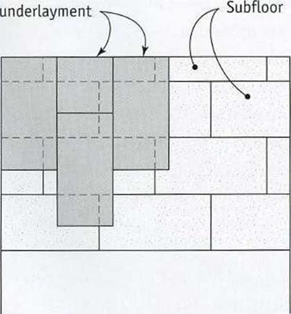
Sheets of underlayment go down just like the subfloor. Lay them so the joints don’t break on the subfloor joints underneath (see the illustration below). When you have to cut a panel to length, lay the cut end against the wall with the factory edges in the middle of the room. This will ensure a tight fit between sheets.

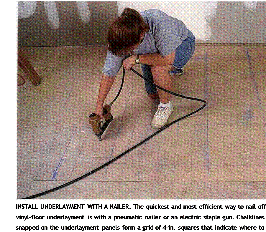
The best way to secure underlayment to the subfloor is with a pneumatic or heavy-duty electric stapler. Drive one staple every 4 in. along the edges of each sheet and 4 in. o. c. in

Interior Trim, Cabinets, Countertops, and Clost

4-ft. by 8-ft. sheets of


Interior Trim, Cabinets, Countertops, and Clost

Install underlayment so the joints do not break, or land, on the subfloor joints below.


4 in.


i— 4 in.


Stapling or nailing pattern for underlayment


Staple or nail at 4 in. o. c. along the edges and in the middle of the sheet.


Подпись:Подпись: Helping HandПодпись: Add character with salvaged doors. A new house gains some wonderful history when it has a few old doors. Interesting, beautifully made old doors can be found at architectural salvage yards and building-supply recyclers.

both directions in the field. If necessary, snap chalklines to make a grid of 4-in. squares. A lot of staples are needed to make sure the underlayment doesn’t bubble should it absorb moisture from the vinyl adhesive or other sources.

If you’re nailing by hand, drive iM-in. ring – shank nails in the same pattern as described above. The problem with nails is that they must be driven exactly flush with the surface of the underlayment. If they are left proud (protruding above the surface), then you’ll be able to see them through the thin vinyl floor­ing. If they’re driven below the surface, they can be covered and hidden with a leveling compound—but that means more work.

After nailing the underlayment in the bath­room, fill the joint between the panel and the bathtub with silicone caulk. This helps prevent water from entering at that junction.

Surface Drainage System

The surface drainage system should remove all flow of rainwater from the road’s sur­face, and from the highway slopes as well as the runoff from adjacent land. Surface drainage systems are also important in the proper management of polluted runoff and in minimizing environmental impacts. The surface drainage can be divided into transverse drainage and longitudinal drainage.

Transverse Drainage – Typically used to allow existing water courses to pass under/over the road which would, otherwise, form a physical barrier. These are normally constructed as aqueducts or culverts (see Chapter 12, Fig. 12.3).

Longitudinal Drainage – The main objective is the fast collection and removal of the rainwater that falls upon the road’s immediate surroundings, and of the water from the adjacent areas, edges, excavation slopes and central reserve. This is funda­mental for maintaining the safety of traffic by eliminating water films and puddles from the road surface (which can result in aquaplaning) at the same time reducing the possibility of water infiltration into the pavement’s layers or foundation, which may reduce its load carrying capability.

Longitudinal surface drainage systems include gutters, channels, ditches, swales, galleries and collectors, complemented by their respective manholes, catchpits and sumps. Surface drainage is not the main topic of this book, so readers should look elsewhere for detailed information on this topic (e. g. Kasibati & Kolkman, 2006).

The transport canals – the magic canal (Lingqu)

In the very same year that the Zhengguo canal came into service, a twelve-year-old child named Zheng ascends to the throne of Qin. Because of all the irrigation works, he soon inherits unprecedented economic power, and he becomes the first emperor.

In 225 BC Zheng uses the Hong canal for the supply of grain to his army, during his gradual advances toward the south.[399] [400] The main grain storage and distribution center becomes established at the junction of this canal and the Yellow River. Later, this virtu­al nerve center will become the imperial granary.

The victory of Zheng over the Chu ends the warring states period in 221 BC. The conqueror takes the imperial name of Shi Huangdi (or Che Houang-ti). His empire includes, in rough terms, the basins of the middle and lower courses of the Yellow River (Huang) and of the Yangtze.

The emperor, seeking to extend the empire even further to the south and conquer the land of Yue (the region of Canton), plans a fluvial assault using oar-powered military junks fitted with attack towers. In 219 BC, he decides to dig a navigation canal both to transport the army and to carry its provisions.

“… the emperor sent the military commander Tu Sui with a force of men in towered ships to sail south and attack the hundred tribes ofYue, and ordered the supervisor Lu to dig a canal to transport supplies for the men so that they could penetrate deep into the region of Yue.”[401] [402]

However the land is mountainous between the Yangtze and the Xi, the river that flows into the Canton sea. The chosen passage is the Xiang river, a southern tributary of the Yangtze that is connected to it through the grand lake Dongling. The Lingqu canal (magic canal) is therefore opened between the Xiang, flowing toward the north, and the Gui (or Kwei), a tributary of the Xi that flows southerly. The canal follows the course

The transport canals - the magic canal (Lingqu)

Figure 8.6 The hydraulic works realized by the Qin in south China. The layout of the branched canals in the Chengdu region is taken from the map of von Richthofen (1877).

of the Li, a minor tributary of the Gui (Figure 8.6).38

An intake on the Xiang River at Xing’an supplies an artificial canal that has an almost horizontal bed, with just enough slope to convey a discharge that is 30% that of the Xiang. This canal flows for about 5 kilometers, to a point near the source of the Li.[403] The Li is channelized to support navigation along some thirty kilometers of its length, as far as the confluence of this small river with the Gui. Alongside the Xiang there is a lateral canal about 3 kilometers long, and with a very modest section: 1 to 2 m deep, and 5 to 8 m wide.

The Xiang intake structure on the Xing’an is obviously inspired by the one built sev­eral decades earlier on the Min River. It includes a separation structure downstream of a dam-spillway in the form of a V. This complex is designed to raise the water level to provide for flow into the canal, and to create a basin in which the current is sufficiently weak to allow boats to be maneuvered – while at the same time providing for the evac­uation of flood waters into the ancient bed of the Xiang. This 3.9-m high dam is called the Tianping dam. Several other weirs on the canal itself provide for further regulation of the water level as well as for floodwater overflow, as explained in the following 12th century description:

“The passengers who travel (on the canal) are terrified at certain locations for, at about 2 li (1 km) from the intake where the “spade head” divides the water and guides one of the branches toward the canal, there is another weir (literally: structure that lets excess water leave). Without this weir, the violent force of the springtime flow would damage the canal’s support wall, and the water would never get to the south. Thanks to this structure, the violence of the water is calmed, the dike is not broken, and the water in the canal flows gently. [….] This is truly what one can call an ingenious device. The canal waters wind around in the district of Xing’an, and people use it to irrigate their fields.”[404]

The transport canals - the magic canal (Lingqu)

Figure 8.7 The magic canal (Lingqu), communication link between the Yangtze and the Xi (map from Needham, Ling, Gwei-Djen, 1971, detailed plan adapted from Zheng (1991) and Schnitter (1994)). The detail of the installation at the right may not be as it was built under Shi Huangdi, for it underwent important renovations in 825 AD under the Tang.

Later on another navigable channel is dug behind the separation structure to facilitate the turning of barges and their passage from one canal to the other (Figure 8.7).

The magic canal is renovated in 825 AD and fitted with single gates (flush locks, a system we discuss further on) on the two canals and possibly also on the channelized Li, to maintain navigability during low-water periods. These flush locks are probably replaced in the 12th century by true chamber locks, with 36 openings in all. The canal is destined to remain in service through all of Chinese history, right up to the present. The completion of this project, along with the canals that had already been created dur­ing the feudal period, created a continuous watercourse – though indirect – that links Canton to Chang’an through the Xi, the Li, the Xiang, the Yangtze, the Huai, and then the Yellow River and the Wei canal.

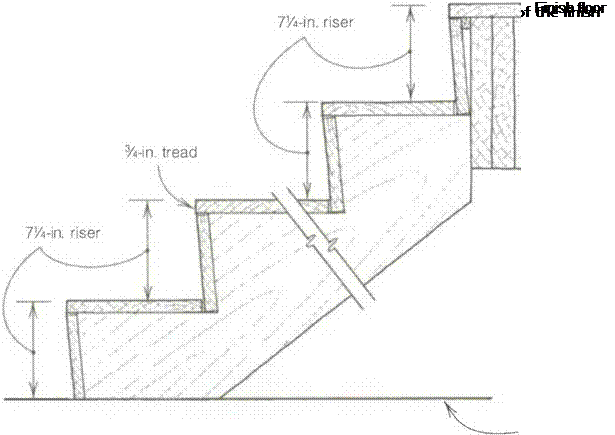
Dropping the stringer

A simple adjustment often needs to be made at the bottom of the stringer to keep the first riser the same height as the rest, because if you nail а 3/нп. board to the first tread, for example, the step increases to 8 in. from JVa in. (see the drawing on the facing page). This is important for safety, because all risers need to be the same height. So subtract the thickness of the finish tread from the bottom of the stringer.

There are many different variations on this detail. If the subfloor is to be car­peted and treads sheathed with 3/ип.

Dropping the stringer

plywood and finished with 3/нп. hard­wood, the stringer has to be dropped by 1Vi in. for every riser to be the same. If the stair is nailed to the subfloor and both treads and subfloor will be covered with 3/4-in. hardwood, nothing has to be done. If the subfloor is sheathed with 3/4-in. hardwood and treads with 3/нп. plywood and 3/s-in. hardwood, drop the stringers by 3/s in. Again, you need to know the exact thickness of the finish floor and tread material before you can frame the stairs.

To help secure the bottom of the stair, lay out a notch for a 2×4 on the bottom front of the first riser. Just take a scrap of 2×4, hold it flush with the outside
corner of the first riser, and scribe around it. This notch will rest on a 2x kicker that is secured to the floor (see the drawing on p. 157).