In all fields of science and engineering, the decision-making process depends on several parameters describing system behavior and characteristics. More often than not, some of these system parameters cannot be assessed with certainty. In a system-optimization model, if some of the coefficients in the constraints
are uncertain, the compliance with the constraints, under a given set of solutions, cannot be ensured with certainty. Owing to the random nature of the constraint coefficients, a certain likelihood that constraints will be violated always exists. The basic idea of chance-constrained methods is to find the solution to an optimization problem such that the constraints will be met with a specified reliability. Chance-constrained formulations have been applied to various types of water resource problems such as groundwater quantity management (Tung, 1986), groundwater quality management (Gorelick, 1982; Wagner and Gorelick, 1987, 1989; Morgan et al., 1993; Ritzel et al., 1994) and monitoring network design (Datta and Dhiman, 1996), reservoir operation (Loucks et al., 1981; Houck, 1979; Datta and Houck, 1984), waste-load allocation (Lohani and Thanh, 1978; Fujiwara et al., 1986, 1987; Ellis, 1987; Tung and Hathhorn, 1990), water distribution systems (Lansey et al., 1989), and freshwater inflow for estuary salinity management (Tung et al., 1990; Mao and Mays, 1994). This section describes the basic properties of chance-constrained models. In the next section an application to waste-load allocation is presented for illustration.
Refer to the general nonlinear optimization problem as stated in Eqs. (8.1a-c). Consider a constraint g(x) < b, with x being a vector of decision variables. In general, decision variables x in an optimization model are controllable without uncertainty. Suppose that some of the parameters on the left-hand-side (LHS) of the constraint g(x) and/or the right-hand-side (RHS) coefficient b are subject to uncertainty. Because of the uncertainty, the compliance with the constraint under a given solution set x cannot be ensured with absolute certainty. In other words, there is a possibility that for any solution x, the constraint will be violated. Consequently, the chance-constrained formulation expresses the original constraint in a probabilistic format as
P [g(x) < b] > a (8.42)
where P [ ] is the probability and a is the specified reliability for constraint compliance. Since this chance-constrained formulation involves probability, it is not mathematically operational for algebraic solution. For this reason, the deterministic equivalent must be derived. There are three cases in which the random elements in Eq. (8.42) could occur: (1) only elements ing(x) are random,
(2) only the RHS b is random, and (3) both g(x) and b are random.
The simplest case is the case 2, where only the RHS coefficient b is random. The derivation of deterministic equivalent of the chance-constraint for this case can be done as follows: The constraint can be rewritten as
P [g(x) < B] > a (8.43)
where B is a random RHS coefficient. Since Eq. (8.43) can be written as then Eq. (8.44) can be expressed as
Fb [g(x)] < 1 – « (8.45)
in which Fb [ ] is the cumulative distribution function (CDF) of random RHS B. The deterministic equivalent of the original chance-constraint Eq. (8.43) can be expressed as
g(x) < b1-a (8.46)
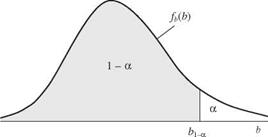
where, referring to Fig. 8.17, b1-a is the (1 – a)th quantile of the random RHS coefficient B satisfying P(B < b1-a) = 1 – a. If the RHS coefficient B is a normal random variable with mean цb and standard deviation ab, Eq. (8.46) can be written as
g(x) < ^b + Z1-aab (8.47)
with z1-a being the (1 – a)th standard normal quantile.
In the case that only the elements in g(x) are random and the distribution functions are known, the chance-constraint can be expressed as
P [G(x) < b] > a (8.48)
For a general nonlinear function G(x), the difficulty lies in the derivations of exact probability distribution and statistical moments of G(x) as functions of unknown decision variables. In this circumstance, statistical moments of G(x) can be estimated by uncertainty-analysis methods such as those described in Tung and Yen (2005). The assessment of the distribution for G(x) is, at best, to be made subjectively. For the sake of discussion, assume that the distribution function of G( x) is known. The deterministic equivalent of the chance-constraint Eq. (8.48) can be expressed as
FG(i>(a) > b (8.49)
|

Figure 8.17 Probability density function of the random right-hand-side coefficient B.
|
where F—yia) is the ath quantile of the random G(x), which is the function of unknown decision variables x. In general, FG(X)(a) in Eq. (8.48) is a nonlinear equation of x even if G(x) is a linear function of x, as will be shown later.
The third case is when both G(x) and the RHS coefficient B are random. The chance-constraint then can be expressed as
P [G(x) – B < 0] > a (8.50)
The deterministic equivalent of Eq. (8.49) can be derived as
Fg^-b (a) > 0 (8.51)
where Fc-(1x)_B (a) is the inverse of the CDF of random G(x) – B taken on the value of a.
As a special case, consider an LP formulation as stated in Eq. (8.3) in which technological coefficients A and/or RHS coefficients b are subject to uncertainty. By imposing a reliability restriction a on the system constraints, the LP model can be transformed into the following chance-constrained formulation:
Maximize c lx (8.52a)
subject to P (Ax < b) > a (8.52b)
In a chance-constrained LP model, the elements in A, b, and c can be random variables. When the objective function coefficient Cj’s are random variables, it is common to replace them by their expected values. Consider the following three cases: (1) elements of the technological coefficient matrix (Aij’s) are random variables, (2) elements of the RHS vector Bi’s are random variables, and
(3) elements Aij and Bi are simultaneously random variables. In the following derivations, it is assumed that random technological coefficients and random RHS coefficient are correlated within a constraint and that these coefficients are uncorrelated between constraints.
Consider that the RHS of the ith constraint Bi is subject to uncertainty. Furthermore, assume that its distribution and statistical moments are known. In this case, the deterministic equivalent of the chance-constraint can be obtained easily from Eq. (8.46) as
n
5^aijXj < bi,1-ai for i = 1, 2,…, m (8.53)
j=1
and the constraint form remains linear.
Consider the case that the technological coefficients aij’s of the ith constraint are random. The deterministic equivalent of the chance-constraint
 P (53 AijXj < bi ) >
j=1
can be derived as (Kolbin, 1977; Vajda, 1972)
n
Y. E(Aij)xj + FzHai)vXCX < bi (8.54)
j=1
where E (Aij) is an expectation of the technological coefficient Aij, Ci is an n x n covariance matrix of n random technological coefficients (Ai 1, Ai2, …, Ain) in the ith constraint, and F—1(ai) is the appropriate quantile for the ai percentage given by the CDF of standardized left-hand-side (LHS) terms. That is,
 LHSi – E(LHSi) Sn=1 AijXj -£n=1 E(Aij)x}
VVar(LHSi)
If all Aij’s are independent random variables, that is, p(Aij, Aij>) = 0, for j = j’, matrix Ci is a diagonal matrix of variances of Aij. To quantify F—1(ai), the distribution of LHS must be known or assumed. Note that the LHSs in an LP model are the sum of several random variables. By the central limit theorem (see Sec. 2.6.1), the random LHS can be approximated as a normal random variable. Therefore, Eq. (8.54) can be written as
E(Aij)Xj + Ф 1(«i)y/x*Cix < bi (8.56)
j=1
with Ф( ) being the standard normal CDF. From Eq. (8.55) one realizes that when Aij’s are random, the resulting deterministic equivalents of the chance constraints are no longer linear functions of the decision variables. The chance – constrained model has to be solved by nonlinear programming algorithms. In the next subsection of application, a sequential LP algorithm is used to linearize Eq. (8.56).
Finally, when both the technological coefficients and the RHS coefficient of the ith constraint are random, the chance-constraint format, referring to Eq. (8.50), can be written as


![DETAILS Подпись: Find a comfortable seat. A small workbench or even a 5-gal. bucket allows you to sit down when installing latches and locksets. [Photo by Don Charles Blom]](/img/1312/image849.gif) Buy your welcome mat early! To reduce the amount of dirt that gets tracked into a house after new carpeting and vinyl and wood flooring have been installed, set up some sort of dirt-catching mat. Put it by the front door near a sign that says, “Please wipe your feet or remove your shoes.”
Buy your welcome mat early! To reduce the amount of dirt that gets tracked into a house after new carpeting and vinyl and wood flooring have been installed, set up some sort of dirt-catching mat. Put it by the front door near a sign that says, “Please wipe your feet or remove your shoes.”![DETAILS Подпись: Use an easier handle. A lever-type door handle is easier to open than a round knob is, especially for older folks and those with arthritis or carpal-tunnel pain. [Photo © Rex Cauldwell]](/img/1312/image850.gif)


