LAYDOWN CONDITIONS

Due to the resistance to compaction provided by the coarse aggregate skeleton, SMA mixtures can cause problems during laydown. Thus in almost all countries that have adopted SMA, some additional requirements on conditions at the work site must be observed, including the appropriate temperature, wind velocity, and the absence of rain.

10.2.1 Minimum Temperature of Air and Underlying Layer

To ensure that weather conditions are acceptable during laydown, the air tempera­ture may be checked often. In many countries, however, air temperature is not as important as the temperature of the course on which the hot mixture is going to be placed. Required laydown conditions frequently hinge on the thickness of the constructed layer, because thick layers cool more slowly, and on the type of binder used, whether modified or unmodified.

Two types of weather conditions may be distinguished in specifications: condi­tions at the time of laying and conditions within 24 hours prior to starting work. Average requirements for the minimum air temperature at the time of placing an SMA mixture range from 5°C to 10°C as exemplified by the following:

• German Dav documents stipulate an air temperature of not less than +5°C (Milster et al., 2004)

• The Czech standard CSN 736121 requires +5°C.

• The Polish guidelines WT2 2008 specify +10°C for courses less than 3 cm thick and +5°C for courses greater than or equal to 3 cm thick.

• The Australian NAS AAPA 2004 calls for +5°C, with the limitation that laying courses thinner than 4 cm or containing a modified binder should be avoided at such low temperatures.

In general, the temperature requirements are becoming stricter (increased) in cases where the thickness of a course is less than 40 mm; for that thickness, a minimum requirement of +10°C is commonly specified. In Germany’s ZTV Asphalt-StB 07, the weather limitations for SMA laying are as follows:

• When the course thickness is less than 3 cm, the minimum air temperature is +10°C, and the minimum sublayer temperature is +5°C.

• When the course thickness is more than 3 cm, the minimum air tempera­ture is 5°C.

The average requirements for the specified underlying layer’s temperatures are similar and are also within a range of 5-10°C. A higher value is often used for mixtures with modified binder. Another document, the U. S. Federal Aviation Administration Advisory Circular 150/5370-10B on civil airfields, has stipulated the following minimum temperatures of the underlying course during laydown, which depend on the thickness of the asphalt course being placed:

• For a course less than 2.5 cm thick, the underlying layer temperature must not be lower than 10°C.

• For a course 2.5-7.5 cm thick, the underlying layer temperature must not be lower than 7°C.

• For a course greater than 7.5 cm thick, the underlying layer temperature must not be lower than 4°C

Slightly lower values than those just cited have been adopted when specifying temperatures during the day directly preceding the start of laying down the hot mix­ture. For example, according to the Czech standard CSN 73 6121, the air temperature must be no less than 3°C (5°C for a thin course), and according to the Polish guide­lines WT2 2008, it must be at least 0°C (5°C for a thin course).

Another, indirect method of specifying temperature requirements is by limit­ing the permissible calendar period of SMA laydown—for example, by imposing a ban on works over a specified period of the year (e. g., between October 15 and March 15).

Finally, it is worth noting that a bituminous mixture with an unmodified binder can be laid down at a temperature slightly lower than a bituminous mixture with a modified binder.

Time-dependent reliability models for hydrosystems

Considering only inherent hydrologic uncertainty. Traditionally, the risk associ­ated with the natural hydrologic randomness of flow or rainfall is explicitly considered in terms of a return period. By setting the resistance equal to the load with a return period of T years (that is, r* = lT), the annual reliability, without considering the uncertainty associated with lT, is 1 – 1/T, that is,

P (L < r *|r * = tT) = 1 – 1/T. Correspondingly, the reliability that the random loads would not exceed r * = lT in a period of t years can be calculated as (Yen, 1970)

Ps(t, T) = (4.108)

For large T, Eq. (4.108) reduces to

Ps(t, T) = exp( t/T) (4.109)

If T > t, Eq. (4.108) can further be approximated simply as ps(t, T) = 1 -1/T.

Considering both inherent hydrologic uncertainty and hydraulic uncertainty. In the

case where the uncertainty of the resistance is not negligible and is to be con­sidered, the annual reliability of a hydrosystem infrastructure then has to be evaluated through load-resistance interference on an annual basis. That is, the annual reliability will be calculated by evaluating P(L < R) as Eq. (4.1), with f L(t) being the probability distribution function of annual maximum load. Hence the reliability of a hydrosystem over a service period of t years can be cal­culated by replacing the term 1/T in Eqs. (4.108) and (4.109) by 1 – P(L < R). Then the results are

Ps(t, L, R) = [P(L < R)]t (4.110)

Ps(t, L, R) = exp{—t x [1 – P(L < R)]} (4.111)

in which the evaluation of annual reliability P (L < R) can be made through the reliability methods described in preceding sections.

Incorporation of a design event. In the design of hydraulic structures, the com­mon practice is to determine the design capacity based on a preselected design return period tT and safety factor SF. Under such a condition, the magnitude of the future annual maximum hydrologic load can be partitioned into two com­plementary subsets, that is, t < tT and t > tT, with each representing different recurrence intervals of the hydrologic process. The reliability of the hydrosys­tem subject to the ith hydrologic load occurring in the future can be expressed by using the total probability theorem (Sec. 2.2.4) as

Ps, i = P (Li < r)

= P(Li < r |Li > tT) P(Li > tT) + P(Li < r |Li < tT) P (Li < tT)

= P (tT < Li < r) + P (Li < r, Li < tT)

= P1 + P 2 (4.112)

where Pi and P2 can be written explicitly as

Time-dependent reliability models for hydrosystems

Подпись: (4.117)

Time-dependent reliability models for hydrosystems
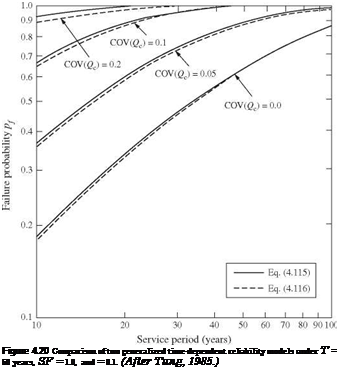
Подпись: Equation (4.115) is based on the binomial distribution for random occurrence of the loads, whereas Eq. (4.116) is based on the Poisson distribution. When hydraulic uncertainty is negligible, Eqs. (4.115) and (4.116) reduce, respectively, to

r

Подпись: Figure 4.20 Comparison of two generalized time-dependent reliability models under T = 50 years, SF = 1.0, and = 0.1. (After Tung, 1985.)

probability computed by the two models converge as the service life increases. Without considering hydraulic uncertainty [i. e., Cov(Qc) = 0], the failure prob­ability is significantly underestimated. Computationally, the time-dependent model based on the binomial distribution, i. e., Eq. (4.39a), is much simpler than that based on the Poisson distribution.

Shingling across a valley

When a porch roof intersects the main roof at a right angle, a valley is formed. Shingles can be laid across a valley in different ways.

A woven valley is formed by weaving shingles across the valley, alternately overlapping from the main roof onto the porch roof, then vice versa. When properly done, a woven valley is watertight. Let each course of shingles overlap the valley by at least 12 in. and keep nails 8 in. or more from the centerline of the valley.

Подпись:Подпись: Save your knees when shingling. A foam pad makes a great cushion when you're nailing roof shingles. If a pad isn't convenient for you to use, try wearing cushioned knee pads. Подпись: iiiiiiiiiiiiiiiiiiiiiiiiiiiiiiiiiiiiiiiiiiiiiiiiiiiiiiiiiiiiiiiiiiiiiiiiiiiiiiiiiiiiiiiiiiiiiiiiiiiiiiiiiiiiiiiiiiiiiiiiiiiiiiiiiiiiiiiiiiiiiiiiiiiiiiiiiiiiiiiiiiiiiAn alternative to a woven valley is a closed, or cut, valley. To create a cut valley, let all shingle courses from the main roof lap across the porch valley by at least 12 in. Don’t alter­nate back and forth from the main roof to the

It’s hard work to hand up sheathing panels.

We yell back and forth from the roof to the ground. Everyone should wear a hard hat.

With some experienced volunteers using nailers and

others hammering, the panels go down quickly.

After lunch, we shift from sheathing to shingling.

The scent of cut wood is replaced by the smell of asphalt; pretty soon, we’re hoisting shingles onto the roof.

Shingling across a valley

Shingling across a valleyporch roof. After the shingles are laid on the main roof, lay the shingles on the porch roof so that each course laps over those on the main roof. Next, snap a chalkline down the center of the valley; use blue chalk, because most other colors stain. Cut the top layer of shingles at this chalkline. I use tinsnips or a utility knife with a hook blade to trim shingles to this line and to avoid cutting the lapped shingles below.

RETAIL STORES

The minimum fixture requirements for retail stores differ from the examples that we have just been working with. However, the concept and approach of computing the needs is same. Refer to Figure 9.3 for listings that pertain to retail stores. You can see that the table is very similar, in layout, to the one we have just been using. Pay particular attention to the number 6 at the heading of retail stores. Refer back to Figure 9.2 for an explanation of the note. You will find that one bathroom facility can be used by both males and females in certain types of occupancies. For example, an office with 1200 square feet, or less, can be served by a single restroom for both sexes. A retail store with 1500 square feet, or less, can also be served by one rest­room, unless the store is classified as a service station. Other types of build­ings that may qualify for a single bathroom are restaurants, self-service laun­dries, beauty salons, and barber shops. In all cases, the use of a single restroom is contingent on the square footage of the building. With this said, let’s run through a sample sizing example.

Assume that our sample building will accommodate 59 people. Use the table in Figure 9.3 to determine the minimum number of plumbing fixtures required. For the purposes of this exercise, assume that the single-bath­room rule is not applicable. Go ahead, run the numbers, and then compare them with mine.

You should have found that the male restroom requires two water closets. A total of three water closets is needed for the female restroom. The male restroom is required to have only one lavatory, but the female restroom is re­quired to have three lavatories. Only one drinking fountain is needed, subject to building design. By this, I mean that a drinking fountain is required on each

Подпись: PLUMBER'S AND PIPE FITTER'S CALCULATIONS MANUAL

200 sq ft

Retail stores6 per person

Persons (total)

Male

Female

1-35

1

1

36-55

1

2

56-80

2

3

81-100

2

4

101-150 For each additional 200

2

5

persons over 150, add

1

1.757


Drinking fountains

Persons (total)

Male

Female

Persons

Fixtures

1-15

1

1

1-100

1

16-35

1

2

101-250

2

36-60

1

3

251-500

3

61-125

2

4

501-1000

4

For each

Not less than one

additional 200

fixture each floor

persons over 125, add

1

1.757

subject to access.


FIGURE 9.3 ■ Minimum fixtures for retail stores. (Courtesy of Standard Plumbing Code)

floor of the building, subject to access. If you did not arrive at these numbers, go over the table again and see if you can find the error in your calculations.

Remedying a Mold Problem

Remedying a Mold Problem

if you think you have a mold problem or if you are sick in your home and suspect mold is to blame, I recommend contacting a reputable professional to do an investigation. The self-test kits found at local hardware stores are not accurate. They may tell you there is a problem when there is not and they are not good at detecting Stachybotrys, one of many problematic types of mold. Stachybotrys has frequently been referred to as "black mold," but there are many types of mold that are black. You can’t judge a mold by its color; there are some types of edible mold that are black and other molds that aren’t black but are probably every bit as bad as if not worse than Stachybotrys. So get­ting a competent diagnosis is important.

Several states have licensing requirements for mold inspectors. By itself, having a license does not make one competent. Ever had a bad hair­
cut from a licensed cosmetologist? A bad roof in­stalled by a licensed roofer? One helpful screening tool is checking to see if the inspector has Errors and Omissions (E & O) insurance. Another is ask­ing for references. See if the consultant has been in the business for awhile, if they have complaints on file with the Better Business Bureau, and if they are in good standing with professional or trade organizations. It also makes sense to hire a mold inspector who has experience in other areas of in­door environmental quality, building science, and Building Biology.

A mold inspection should really be called a mold investigation. Unless you see mold there won’t be any inspecting, and at least half the time mold is hiding. One way to look for mold is look for damp spots. The inspector should spend time checking the moisture levels of walls and ceilings
control procedures more complicated and re­quires site – and climate-specific design strate­gies beyond the scope of this book. Guides that distinguish and explain these design strategies for climate-based moisture control are avail­able through The Energy & Environmental Building Association (EEBA). We highly rec­ommend them. (See Further Reading at the end of this chapter.)

Insulation Products

Time-dependent reliability models

Reliability computations for time-dependent models can be made for determin­istic and random cycle times. The development of a model for deterministic cycles is given first, which naturally leads to the model for random cycle times.

Number of occurrences is deterministic. Consider a hydrosystem with a fixed resistance (or capacity) R = r subject to n repeated loads L1, L2,…, Ln. When the number of loads n and system capacity r are fixed, the reliability of the system after n loadings ps(n, r) can be expressed as

Ps(n, r ) = P [(L1 < r ) n (L2 < r ) П—П (Ln < r )] = P (Lmax < Г ) (4.100)

where Lmax = max{L1, L2,…, Ln}, which also is a random variable. If all ran­dom loadings L are independent with their own distributions, Eq. (4.100) can be written as

Ps(n, r) = [FLi(r)] (4.101)

i=1

where FLi (r) is the CDF of the ith load. In the case that all loadings are gener­ated by the same statistical process, that is, all Ls are identically distributed with FLi(r) = FL(r), for i = 1, 2,…, n, Eq. (4.101) can further be reduced to

Подпись: (4.102)Ps(n, r) = [FL(r )]

Подпись: Ps(n) Time-dependent reliability models Подпись: (4.103)

If the resistance of the system also is a random variable, the system reliability under the fixed number of loads n can be expressed as

Number of occurrences is random. Since the loadings to hydrosystems are re­lated to hydrologic events, the occurrence of the number of loads, in general, is uncertain. The reliability of the system under random loading in the specified time interval [0, t] can be expressed as

TO

Подпись: (4.104)Ps(t) = n (t |n) Ps(n)

n=0

in which n(t |n) is the probability of n loadings occurring in the time interval [0, t]. A Poisson distribution can be used to describe the probability of the num­ber of events occurring in a given time interval. In fact, the Poisson distribution has been found to be an appropriate model for the number of occurrences of hy­drologic events (Clark, 1998; Todorovic and Yevjevich, 1969; Zelenhasic, 1970). Referring to Eq. (2.55), n(t |n) can be expressed as

e Xt ( X t )n

n (t |n) =————- (— (4.105)

n!

where X is the mean rate of occurrence of the loading in [0, t], which can be estimated from historical data.

Substituting Eq. (4.105) in Eq. (4.104), the time-dependent reliability for the random independent load and random-fixed resistance can be expressed as

Подпись: e Xt (Xt)n" n! Подпись: Ps(t) = n= 0 Подпись: Ps (n, r) fR (r) drПодпись: 0(4.106)

Under the condition that random loads are independently and identically dis­tributed, Eq. (4.106) can be simplified as

n TO

Ps (t) = e- t [1-FL(r)] fR (r) dr (4.107)

0

Interior walls

Once the exterior wall lines are accu­rately in place, you can measure off them to get the location of interior walls. Just keep an eye on the plans to get the dimensions right.

Laying out the long interior walls next makes it easier to locate and mark all the short, 2×4 walls that make up closets and bathrooms. Watch the floor plan. It may show that an interior bedroom wall is 12 ft. 7 in. from the outside of the building to the center of the 2×4 wall. Because half of ЗУ2 in. is 13A in., add 13/д in. to 12 ft. 7 in. to get the overall dimension of this wall, which is 12 ft.

83/д in. from outside to outside.

Measure in this distance from the out­side of the exterior wall of the slab or floor deck, mark it, and place an X to the inside of the mark, as shown in the drawing on the facing page. Do this at both ends of the wall and connect the marks with a chalkline. The location of the X is important because it indicates the exact location of the wall. Placing the X on the wrong side of the mark can be disastrous. Imagine the excite­ment of a plumber, for example, trying to install a bathtub in a room that is ЗУ2 in. too narrow.

You might find that plans don’t always have the exact measurements you need. For example, floor plans might show a 60-in. dimension in a bathroom to accommodate a standard-size bathtub.

In reality, what is needed is 601Л in. so that the tub will actually fit without hav­ing to carve up the walls. And because
of the size of plumbing drains and vents, it’s best to build bathroom walls out of 2x6s to accommodate the plumbing.

PLATING

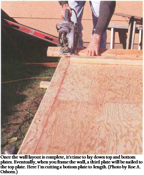
Once you’re finished with the wall – layout chalklines, you can begin to lay down the top and bottom plates. Eventually, when you frame the wall, a third plate will be nailed to the top plate to hold the walls together. At times, when doing remodeling work, I have opened up a wall to find that only a sin­gle top plate was used. This allowed the walls to separate, opening up cracks in the plaster and siding, because they were not tied together with the double top plate.

Pick long, straight stock for plates, which makes it easier to keep walls straight once they’re raised upright.

Plate the long outside walls (called

Подпись:through walls) first. Shorter walls that intersect the through walls are called butt walls. These can be plated once the through walls are in place. Get the long borders of a house in place, and the shorter inside pieces fit together easier.
Placing and securing plates

Remember that top and bottom wall plates are placed flush with the chalk­lines on the X side of the marks made on the deck. But these plates need to be cut accurately or the walls won’t end up square and plumb. Again, begin with the outside walls. Lay down a long 2x plate on the chalkline, cut it to length,
and tack it in place with two or three 8d nails. Run your plates continuously, ignoring door and window openings.

The bottom plate in doorways will be cut out later.

Plating on a slab

Plating on a concrete slab requires a slightly different approach than plating on a wooden floor system. Slabs nor­mally have anchor bolts located around the perimeter to hold the exterior walls in place. On interior walls, the plates are held in position by a hardened screw or nail or by actually shooting a steel pin through them into the con­crete. However you do it, you can’t easily tack the plates in place like you can on a wooden deck. Just position the bottom plate on the line and tack the top plate to it.

Don’t forget to use pressure-treated wood for plates that are in direct contact with concrete. Anyone who has done remodeling work can tell stories of termite-ridden sills or plates made of untreated lumber. If termites get by the sills or plates, they start eating toward the attic. That’s why, in Hawaii (home to the mother of all termites), entire frames are often made of treated wood.

Where there are anchor bolts, their location can be marked on the plate in the same manner as with sill plates (see Chapter 4).

Modeling intensity and occurrence of loads

A hydraulic structure placed in a natural environment over an expected ser­vice period is subject to repeated application of loads of varying intensities. The magnitude of load intensity and the number of occurrences of load are, in gen­eral, random by nature. Therefore, probabilistic models that properly describe the stochastic mechanisms of load intensity and load occurrence are essential for accurate evaluation of the time-dependent reliability of hydrosystems.

Probability models for load intensity. In the great majority of situations in hy­drosystems reliability analysis, the magnitudes of load to be imposed on the system are continuous random variables. Therefore, univariate probability dis­tributions described in Sec. 2.6 potentially can be used to model the intensity of a single random load. In a case in which more than one type of load is considered in the analysis, multivariate distributions should be used. Some commonly used multivariate distribution models are described in Sec. 2.7.

The selection of an appropriate probability model for load intensity depends on the availability of information. In a case for which sample data about the load intensity are available, formal statistical goodness-of-fit tests (see Sec. 3.7) can be applied to identify the best-fit distribution. On the other hand, when data on load intensity are not available, selection of the probability distribution for modeling load intensity has to rely on the analyst’s logical judgment on the basis of the physical processes that produce the load.

Probability models for load occurrence. In time-dependent reliability analysis, the time domain is customarily divided into a number of intervals such as days, months, or years, and the random nature of the load occurrence in each time interval should be considered explicitly. The occurrences of load are discrete by nature, which can be treated as a point random process. In Sec. 2.5, basic features of two types of discrete distributions, namely, binomial and Poisson distributions, for point process were described. This section briefly summarizes two distributions in the context of modeling the load-occurrences. Other load – occurrence models (e. g., renewal process, Polya process) can be found elsewhere (Melchers, 1999; Wen, 1987).

Bernoulli process. A Bernoulli process is characterized by three features:

(1) binary outcomes in each trial, (2) constant probability of occurrence of out­come in each time interval, and (3) the outcomes are independent between trials. In the context of load-occurrence modeling, each time interval repre­sents a trial in which the outcome is either the occurrence or nonoccurrence of the load (with a constant probability) causing failure or nonfailure of the sys­tem. Hence the number of occurrences of load follows a binomial distribution, Eq. (2.51), with parameters p (the probability of occurrence of load in each time interval) and n (the number of time intervals). It is interesting to note that the number of intervals until the first occurrence T (the waiting time) in a Bernoulli process follows a geometric distribution with the PMF

g(T = t) = (1 – p)t-1 p (4.97)

The expected value of waiting time T is 1/p, which is the mean occurrence period. It should be noted that the parameter p depends on the time interval used.

Poisson process. In the Bernoulli process, as the time interval shrinks to zero and the number of time intervals increases to infinity, the occurrence of events reduces to a Poisson process. The conditions under which a Poisson process applies are (1) the occurrence of an event is equally likely at any time instant,

(2) the occurrences of events are independent, and (3) only one event occurs at
a given time instant. The PMF describing the number of occurrences of loading in a specified time period (0, t] is given by Eq. (2.55) and is repeated here:

e Xt ( Xt )x

Px (xX, t) =—— for x = 0,1, …

x!

in which X is the average time rate of occurrence of the event of interest. The interarrival time between two successive occurrences is described by an expo­nential distribution with the PDF

ft(tX) = Xe-t for t > 0 (4.98)

Although condition (1) implies that the Poisson process is stationary, it can be generalized to a nonstationary Poisson process, in which the rate of occurrence is a function of time X(t). Then the Poisson PMF for a nonstationary process can be written as

Подпись: (4.99)P(x = x) [/0 x(t) d t]x exp [-/0 x(t) d t]

x!

Equation (4.99) allows one to incorporate the seasonality of many hydrologic events.

Other Techniques for Discharging Mixture

Special self-propelled hoppers (e. g., MTVs) have been used to avoid segregation dur­ing the discharge of a mixture from the dump truck to the paver hopper and to minimize the risk of placing cool mixture (by remixing). These mobile machines operate between the dump truck and the paver to eliminate any contact between the two. MTVs are equipped with conveyors to transport the mixture to the paver hop­per. These devices eliminate jarring of the paver caused by contact with the delivery trucks or by the mass of mix dropping into the hopper. They hold a larger mass of material than a paver hopper, which helps to keep the temperature high, and allows the paver to keep moving forward. Another advantage of MTVs is the possibility of remixing the mixture constituents. This eliminates the risk of segregation and

image94

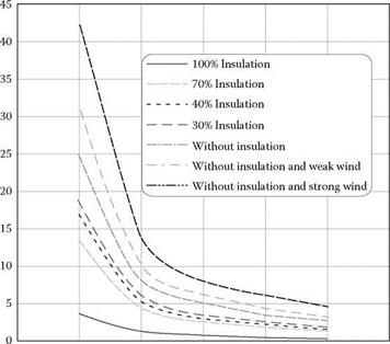
0 5 10 15 20 25 30

Haul truck loading, Mg

FIGURE 10.3 Impact of load capacity and applied insulation of the truck bed on the tem­perature drop of mixture in various weather conditions. (From Spuziak, W., Proceedings of the 6th International Conference Durable and Safe Road Pavements, Kielce, Poland, 2000. With permission.)

enables the breaking of large lumps of cool mixture that may occur during trans­portation. Then the mixture is transferred to the paver hopper using a conveyor belt. MTVs are especially useful when laying mixtures susceptible to segregation and paving during cooler periods of the year (see Chapter 11, Section 11.8).

Hydraulics in the Roman empire: Driving Force of development and symbol of civilization

The Etruscan hydraulic heritage and the beginnings of Rome

Civilization does not truly begin to develop in the western Mediterranean until the begin­ning of the 8th century BC. This begins according to the legend when the Phoenicians, led by Elissa, princess of Tyr, found Carthage on the Tunisian coast. Then the Greeks establish colonies in Sicily and in the south of the Italian peninsula in the middle of the 8th century BC. These colonies become a cultural ensemble called Greater Greece. But the capital event for Italy during this same period is the arrival of yet another people who settle to the north of the Tiber. According to Herodotus, these new arrivals came from Anatolia. In response to an extended period of famine, the king of the Lydians has his son Tyrrhenios lead half of his people out of their homeland. They take to the sea, trav­eling westward to Tuscany and Umbria where they become a new people: The

Etruscans – or the Tyrrhenians as they are called by the Greeks. In the 6th century BC they spread onto the plain of the river Po, and to the south as far as Campania. Their beautiful urban civilization profoundly marks the Italian countryside; the cities have their own water supply, the streets are straight and aligned at right angles, with gutters and extended underground sewage networks, following the Aegean and Oriental tradi­tions. The Etruscan economic miracle rests on three pillars: the mastery of commerce, the exploitation of iron mines, and the development of land for agriculture.

The principal obstacle to development of Etruria is the accumulation of water in the numerous marshy depressions of the valleys. During the entire period from the 7th to the 4th century BC, the Etruscans drain large regions of Italy by means of dense net­works of underground drainage galleries, called cuniculi.1 These galleries, from 300 m to several kilometers in length, are about 1.5 m high and 0.5 m wide. They normally fol­low the courses of the valleys they drain, aligned slightly off the valley centerline (and usually to the right) at a depth of some 30 meters. Vertical shafts are regularly spaced at 30 to 35 m, extending from the galleries up to the surface. These shafts facilitate the ini­tial digging of the drainage galleries, and then provide aeration. These cuniculi follow the valley down to its mouth, or sometimes pass under a ridge to connect to a neighbor­ing valley.

This preoccupation with land drainage is accompanied by a need to control the sup­ply to, and level of, the many lakes of Etruria. Underground drainage works are built in the lakes of Burano, Nemi (near Rome), and Albano. Lake Albano has a 1.5 m wide tun­nel that varies in height from 2 to 3 m. It is 1,200 m long, and passes underneath the present city of Castel Gandolfo. There are also artificial reservoirs, excavated and then sealed through paving with a mixture of clay and chalk. These reservoirs are used in the [208] wet season to store water, and in the dry season to supply water for crops through terra­cotta pipelines.[209]

In their conception and construction of underground conduits, the Etruscans show a marvelous mastery and skill in hydraulic works. They are also good miners. Their know-how in both areas could well have been developed locally, but they surely brought much of their expertise in hydraulics from the Orient. It is interesting to note certain similarities between the Etruscan cuniculi and the qanat, broadly spread within the Persian Empire for water supply (see Chapter 2, Figure 2.19). Recall too that the Mycenaeans used natural grottos to drain marshy depressions (see Chapter 4, in partic­ular Figure 4.10).

The Etruscans are not only miners and peasants, but also sailors: they give their name to the Tyrrhenian Sea. In the 6th century BC, they share maritime domination of the western Mediterranean with the Carthagenians. Their united forces defeat the Phoenicians of Massilia (Marseilles) at the naval battle of Aleria (in Corsica), in about 535 BC. Maritime commerce flourishes, and numerous ports are developed. But in 474 BC, the Syracuse fleet defeats the Etruscans, pushing their maritime commerce back toward the Adriatic. The large port of Spina on the Adriatic is built on a lagoon that is connected to the sea, some 3 km distant, by a 30-m wide canal. It is likely that this port resembled modern Venice, with its canals connecting to the sea and to the nearby estu­ary of the Po.[210]

Simple huts occupy the site of the seven hills of Rome From the 8th century BC, around the marshy depression where the forum will later be built. This site, at the south­ern boundary of Etruria, is easily fortified, and the Tiber River, navigable by small boats, adds to the attractiveness of the site. It is here that one finds the first ford of the Tiber, and soon the first bridge, that of Sublicius. In 575 BC, a city is founded here by Tarquin (Tarquin the Elder), a rich Etruscan.

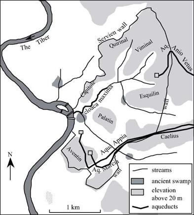
Quite logically, the first hydraulic project in the city is a drainage canal (Figure 6.1). Tarquin the Elder constructed the cloaca maxima to drain the depression of the forum and reclaim its land. At the end of the 6th century BC, Tarquin the Superb, third and last of the Etruscan kings of Rome, had the cloaca Maxima covered over since its physical presence had become an obstacle to further development of the city. With this, the canal began to also serve as a sewer. It had been generously dimensioned by its initial builders, and was not further modified until the 1st century BC under Augustus. Pliny the Elder left us a few words describing this work:

“(…) there are seven rivers, made, by artificial channels, to flow beneath the city. Rushing onward, like so many impetuous torrents, they are compelled to carry off and sweep away all the sewerage; and swollen as they are by the vast accession of the pluvial waters, they rever­berate against the sides and bottom of their channels. Occasionally, too, the Tiber, overflow­ing, is thrown backward in its course, and discharges itself by these outlets: obstinate is the contest that ensues within between the meeting tides, but so firm and solid is the masonry, that it is enabled to offer an effectual resistance.”[211]

Hydraulics in the Roman empire: Driving Force of development and symbol of civilization

Figure 6.1 The city of Rome under the Republic, the cloaca maxima, and the arrival into the city of the first aqueducts. The Aqua Applia passes underneath the Aventin. The Marcia, carried on arches in the countryside, is at a higher elevation, and arrives at Aventin through the siphon of Caelius.

Rome became a republic in about 509 BC, Tarquin having been run out. After the incursion of the Gaels into Italy, about 390 BC, Rome becomes the main power of cen­tral Italy. The Aqua Appia, first of the Roman aqueducts, is built in 312 BC. Its dimen­sions are similar to those of the Etruscan cuniculi (0.69 m by 1.69 m), and almost all of it is buried:

“For 441 years after the founding of Rome, the Romans made do with water that they drew from the Tiber, from wells, or springs. The memory of the springs is still a fond one today. (….) Under the consulship of M. Valerius Maximus and of Pl. Decius Mus, thirty years after the start of the Samnite war, the Aqua Appia was brought into the city by the censor Appius Claudius Crassus, later known as Caecus (The Blind). He is the one who also established the Appian Way from the Capene Gate to the city of Capua. (….). The Appia is fed from a loca­tion in a domain of Lucullus, on the Praenestina road, between the seventh and eighth milles. (…). From the saline spring, a named place near the Porta Trigemina, the conduit has a length of 11,190 paces, of which 11,130 are an underground canal, and, above ground, on support­ing walls and arcades, 60 paces near the Capene Gate.”[212]