Optimal stochastic waste-load allocation

Deterministic waste-load allocation model. Although any number of pollutants may be considered in the overall quality management of a river system, in this example, application a biochemical oxygen demand-dissolved oxygen (BOD-DO) water-quality model is considered.

In LP format, the deterministic WLA model considered herein can be written as

N

Подпись:Maximize ^^( Bj + Dj)

j=i

subject to

1. Constraints on water quality:

aoi + ®ij Bj + ^ ttij Dj < DOsat – DOfd for i = 1,2,…, M (8.59b)

j=1 j=1

2.

Подпись: BL_BjL Ij j Подпись: < Ea for j = j' Подпись: (8.59c)

Constraints on treatment equity:

3. Constraints on treatment efficiency:

Подпись:Подпись:Bj

e-j < 1 – T <e j

j

where Bj, Dj, and Ij are the effluent waste concentrations (mg/L BOD), ef­fluent DO deficit concentration (mg/L), and raw waste influent concentration (mg/L BOD) at discharge location j, respectively, and N is the total number of waste dischargers. The LHS coefficients aoi, ®ij, and Uij in Eq. (8.59b) are
the technological transfer coefficients relating impact on DO concentrations at downstream locations i resulting from the background waste and waste input at an upstream location j. These technological transfer coefficients are functions of water-quality parameters such as reaeration and deoxygenation rates, flow velocity, etc. DOistd and DOisat represent the required DO standard and saturated DO concentration at control point i, respectively. Finally, Ea is the allowable dif­ference (i. e., equity) in treatment efficiency between two waste dischargers, and e_j and e j are the lower and upper bounds of waste-removal efficiency for the j th discharger, respectively. The importance of incorporating the treatment equity in the WLA problems is discussed by many researchers (Gross, 1965; Loucks et al., 1967; Miller and Gill, 1976; Brill et al., 1976; Chadderton et al., 1981).

The water-quality constraint relating the response of DO to the effluent waste can be defined by water-quality models such as the Streeter-Phelps equation (Streeter and Phelps, 1925) or its variations (Dobbins, 1964; Krenkel and Novotny, 1980). To demonstrate the proposed methodologies, the original Streeter-Phelps equation is used herein to derive the water-quality constraints. Expressions for &ij and Uij, based on the Streeter-Phelps equation, are shown in Appendix 8A. The Streeter-Phelps equation for DO deficit is given as follows:

Dx = TKdL0, (e-KdX/U – e-K“x/U) + Doe-Kax/U (8.60)

where Dx is the DO deficit concentration (mg/L) at stream location x (mi), Kd is the deoxygenation coefficient for BOD (days-1), Ka is the reaeration-rate coefficient (days-1), L0 is the BOD concentration at the upstream end of the reach (that is, x = 0), D0 is the DO deficit concentration at the upstream end of the reach, and U is the average streamflow velocity in the reach (mi/day).

Chance-constrained waste-load allocation model. The deterministic WLA model presented in Eqs. (8.59a-d) serves as the basic model for deriving the stochastic WLA model. Considering the existence of uncertainty within the stream envi­ronment, the water-quality constraints given by Eq. (8.59b) can be expressed probabilistically as

Optimal stochastic waste-load allocationПі Пі j

aoi + X) ©ij Bj + 53 Uij Dj < DOsat – DOfd> ai for і = 1,2,…, M

j=1 j=1 )

(8.61)

Based on Eq. (8.53), the deterministic equivalent of Eq. (8.60) can be derived as

Optimal stochastic waste-load allocation

Пі Пі ____________________________________

]T E (©ij) Bj +53 E (Qij) Dj + Fzai V( B, D)‘ C (0f, )(B, D) < Ri


j =1


j =1


(8.62)

in which Ri = DOSat – DOfd – E(a0i), (B, D) is the column vector of BOD and DO deficit concentrations in waste effluent, and C (©i, Qi) is the covariance matrix associated with the technological transfer coefficients in the ith water – quality constraint, including a0i. The stochastic WLA model to be solved consists of Eqs. (8.58a), (8.62), (8.58c), and (8.58d).

Assessments of statistical properties of random technological coefficients. To solve the stochastic WLA model, it is necessary to assess the statistical properties of the random LHS in the chance-constraint Eq. (8.62). As shown in Appendix 8A, the technological transfer coefficients &ij and Uij are nonlinear functions of the stochastic water-quality parameters that are cross-correlated among them within each stream reach and spatially correlated between stream reaches. Furthermore, the complexities of the functional relationships between these transfer coefficients and the water-quality parameters increases rapidly as the control point moves downstream. Hence the analytical derivation of the statistical properties of &ij and Uij becomes a formidable task given even a small number of reaches. As a practical alternative, simulation procedures may be used to estimate the mean and covariance structure of the random techno­logical coefficients within a given water-quality constraint.

The assumptions made in the Monte Carlo simulation to generate water – quality parameters in all reaches of the stream system are as follows: (1) The representative values for the reaeration coefficient, deoxygenation coefficient, and average flow velocity in each reach are second-order stationary; i. e., the spatial covariance functions of water quality-parameters are dependent only on the “space lag” or separation distance; (2) correlation between the reaeration coefficient and average flow velocity exists only within the same stream reach; (3) background DO and BOD concentrations at the upstream end of the entire stream system are independent of each other and of all other water-quality parameters; and (4) all water-quality parameters follow a normal distribution.

In the simulation, variance-covariance matrices representing the spatial cor­relation of a water-quality parameter can be derived from the variogram models (Journel and Huijbregts, 1978) in the field of geostatistics. Three commonly used variogram models are:

1. Transitive variogram model:

Optimal stochastic waste-load allocation(8.63)

2. Spherical variogram model:

Optimal stochastic waste-load allocation(8.64)

3.

Подпись: Cov(|h|) = a2 Подпись: exp Подпись: -|h|2 2h2 Подпись: (8.65)

Gaussian variogram model:

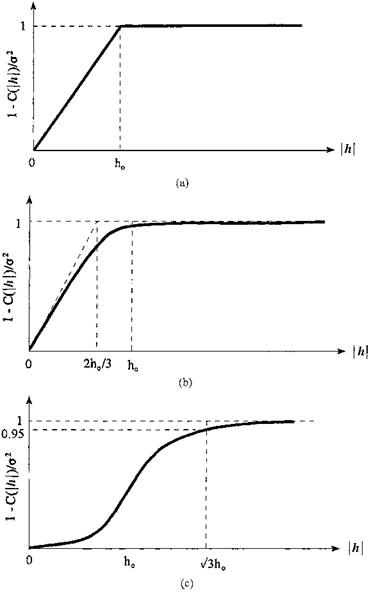
in which Cov(|h|) represents the value of covariance between two measure­ments of the same water-quality parameter separated by a distance h | apart, ho is the length of zone of influence, and a2 is the variance of the water – quality parameter within a given reach. The value of correlation coefficient p(|h|) can be calculated as p(|h|) = Cov(|h|)/a2. When the distance between reaches exceeds ho, the value of the covariance function goes to zero, and the corresponding correlation coefficient is zero as well. Graphically, the three variogram models are shown in Fig. 8.18.

Подпись: R(Ka, U) Подпись: R Ka, Ka RU, Ka Подпись: R Ka,U RU ,U Подпись: (8.66)

To illustrate the concept, consider the water-quality parameters’ reaeration coefficient Ka and average flow velocity U. From the variogram models, the correlation matrix for the two parameters can be constructed as follows:

in which Ka = (Ka, i, Ka2,…, Ka N) and U = (Ui, U2,…, UN) are vectors of the reaeration coefficient and average velocity in each stream reach, respec­tively (see Fig. 8.19). In Eq. (8.66), R(Ka, Ka), R(Ka, U), R(U, U) are N x N square symmetric correlation matrices, with N being the number of stream reaches in the WLA model. Submatrices R(Ka, Ka) and R(U, U) define the spa­tial correlation of Ka and U between the reaches, whereas submatrix R(Ka, U) defines the cross-correlation between Ka and U within the same reach. Under assumption 2 previously mentioned, the submatrix R(Ka, U) is a diagonal ma­trix. For water-quality parameters that are not cross-correlated with other pa­rameters but are spatially correlated, the associated correlation matrix has a form similar to R(U, U). For parameters that are spatially independent, their correlation matrices are in the form of an identify matrix. Once the correlation matrix of normal stochastic parameters within a reach and between reaches is established according to the specified variogram model, generation of stochastic water-quality parameters can be obtained easily by the procedures for gener­ating multivariate random variates described in Sec. 7.5.2.

In summary, the simulation for generating spatially and cross-correlated water-quality parameters can be outlined as the follows:

1. Select an appropriate variogram model for a given water-quality parameter, and construct the corresponding covariance matrix C or correlation matrix R.

2. Apply procedures described in Sec. 7.5.2 to obtain the values of the water – quality parameter for each reach in the WLA model.

3. Repeat steps 1 and 2 for all water-quality parameters.

Optimal stochastic waste-load allocation

Figure 8.18 Variograms of different types: (a) transitive model; (b) spherical model; (c) Gaussian model.

°(Kai, Kai)

*(Kai, Ka2 ) –

*(Kai, KaN )

*(Kai, Ui) 0 •••

0

* (Ka2,Kai)

*(Ka2, Ka2) –

*( K^ KaN )

G(Kai, Kai) 0 •"

0

*( KaN, Kai)

*(KaN, Ka2 ) –

*(KaN, KaN )

0

0 •••

*(KaN, Un )

*(Ul, Kai)

0 •••

0

*(Ui, Ui)

o(Ux, U 2)

••• a(Ui, UN)

0

*(U 2 , Ka2) …

0

a(U 2. K)

*(U2 ,U 2)

•• • <y(U1 , Un )

0

0 •••

*(Un, KaN )

a(UN, U i) a(UN, U 2)

••• *(Un, Un )_

Figure 8.19 Structure of covariance matrix C (Ka, U) for N – reach stream system.

For each set of the water-quality parameters generated by steps 1 through 3, the values of the technological coefficients are computed. Based on the simu­lated values, the mean and covariance matrices of the random technological coefficients for each water-quality constraint are calculated and used in solving the stochastic WLA problem. The simulation procedure described in this sub­section to account for spatial correlation is called unconditional simulation in the field of geostatistics (Journel and Huijbregts, 1978).

Technique for solving an optimal stochastic WLA model. The deterministic WLA model presented previously follows an LP format and can be solved using the simplex algorithm. However, the deterministic equivalents of the chance – constrained water-quality constraints are nonlinear. Thus the problem is one of nonlinear optimization, which can be solved by various nonlinear programming techniques mentioned in Sec. 8.1.2.

In this example, linearization of the chance-constrained water-quality constraints is done, and the linearized model is solved iteratively using the LP simplex technique. More specifically, the algorithm selects an assumed solution to the stochastic WLA model that is used to calculate the value of the nonlinear terms in Eq. (8.62). The nonlinear terms then become constants and are moved to the RHS of the constraints. The resulting linearized water-quality constraints can be written as

E(®ij)Bj + E(Qij)Dj < Щ – F-1(at) (B, t»tC(&t, )(B, D)

j=1 J =1

(8.67)

in which B and D are assumed solution vectors to the stochastic WLA model.

The linearized stochastic WLA model, replacing Eq. (8.62) by Eq. (8.67), can be solved using LP techniques repeatedly, each time updating the previous

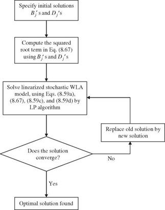
solution values with those obtained from the current iteration, resulting in new values for the RHS. The procedure is repeated until convergence criteria are met between any two successive iterations. A flowchart depicting the procedures is given in Fig. 8.20. Of course, alternative stopping rules could be incorporated in the algorithm to prevent excessive iteration during the computation. Prior to the application of these solution procedures, an assumption for the distribution of the random LHS must be made to determine the appropriate value for the term Fz(ai) in Eq. (8.67).

Owing to the nonlinear nature of the stochastic WLA model, the global op­timum solution, in general, cannot be guaranteed. It is suggested that a few runs of the solution procedure with different initial solutions be carried out to ensure that the model solution converges to the overall optimum. A reasonable initial solution is to select the waste effluent concentration for each discharger associated with the upper bounds of their respective treatment levels. By doing so, the initial solution corresponds to waste discharge at their respective lower

Optimal stochastic waste-load allocation

Figure 8.20 Flowchart for solving linearized chance-constrained WLA model.

limits. If the stochastic WLA solution is infeasible during the first iteration, it is likely that the feasible solution to the stochastic WLA problem does not exist. Hence time and computational effort could be saved in searching for an optimal solution that might not exist.

Numerical example. The preceding chance-constrained WLA model is applied to a six-reach example shown in Fig. 8.21. The means and standard deviations for the water-quality parameters in each reach are given in Tables 8.5 and 8.6 based on the data reported in the literature (Churchill et al., 1962; Chadderton et al., 1982; Zielinski, 1988).

To assess the mean and correlation matrix of the random technological co­efficients in the water-quality constraints, the Monte Carlo simulation proce­dure described in Sec. 6.5.2 is implemented to generate multivariate normal water-quality parameters. Different numbers of simulation sets are generated to examine the stability of the resulting means and covariance matrix of the technological coefficients. It was found that the statistical properties of ©ij and Uij become stable using 200 sets of simulated parameters. In the exam­ple, a positive correlation coefficient of 0.8 between the reaeration coefficient and average flow velocity is used. Both normal and lognormal distributions are assumed for the random LHS of the water-quality constraints

Пі Пі

a0i + 53 ©i> + 53 ^ij Dj (8.68)

j=1 j=1
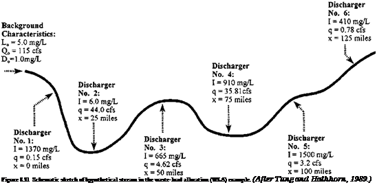
Подпись: Figure 8.21 Schematic sketch of hypothetical stream in the waste-load allocation (WLA) example. (After Tung and Hathhorn, 1989.)
in Eq. (8.67). Various reliability levels ai ranging from 0.85 to 0.99 for the water-quality constraints are considered.

TABLE 8.5 Mean Values of Physical Stream Parameters Used in WLA Example

(a) Mean stream characteristics for each reach

Reach

Deoxygenation coefficient Kd (L/day)

Reaeration coefficient Ka (L/day)

Average stream velocity (mi/day)

Raw waste concentration I (mg/L BOD)

Effluent flow rate (ft3/s)

1

0.6

1.84

16.4

1370

0.15

2

0.6

2.13

16.4

6.0

44.00

3

0.6

1.98

16.4

665

4.62

4

0.6

1.64

16.4

910

35.81

5

0.6

1.64

16.4

1500

3.20

6

0.6

1.48

16.4

410

0.78

(b) Background characteristics

Upstream

Upstream

Upstream

waste concentration

flow rate

DO deficit

L0 (mg/L BOD)

Q0 (ft3/s)

D0 (mg/L)

5.0

115.0

1.0

In the example, the length of each reach in the system is 10 mi, and the spatial correlation of representative water-quality parameter values between two reaches is computed based on the separation distance between the centers of the two reaches. To examine the effect of spatial correlation structure on the optimal waste-load allocation, two zones of influence (ho = 15 mi and ho = 30 mi) along with the three variogram models, Eqs. (8.63) through (8.65), are used. A value of ho = 15 mi implies that the water-quality parameters in a given reach are spatially correlated only with the two immediate adjacent reaches. For ho = 30 mi, the spatial correlation extends two reaches upstream and downstream of the reach under consideration. The optimal solutions to the stochastic WLA problem under these various conditions are presented in Tables

8.7 and 8.8.

TABLE 8.6 Standard Deviations Selected for Physical Stream Characteristics

(a) For each reach

Reach

Deoxygenation coefficient

Reaeration coefficient

Average stream velocity

(units)

Kd (L/day)

Ka(L/day)

U(ft3/s)

1-6

0.2

0.4

4.0

(b) Background characteristics

Upstream

Upstream

Upstream

waste concentration

flow rate

DO deficit

L0(mg/L BOD)

Qo(ft3/s)

Do (mg/L)

10.0

20.0

0.3

TABLE 8.7 Maximum Total BOD Load that Can Be Discharged for Different Reliability Levels and Spatial Correlation Structures under Normal Distribution

a

I *

ho

= 15 mi

ho = 30 mi

T

S

G

T

S

G

0.85

671t

734

737

679

659

664

694

0.90

633

693

695

639

624

625

656

0.95

588

644

646

593

580

578

610

0.99

521

570

572

524

516

511

541

* I = independence; T = transitive model; S = spherical model; G = Gaussian model.

t Total BOD load concentration in mg/L.

Examining Tables 8.7 and 8.8, the maximum total BOD discharge, under a given spatial correlation structure, reduces as the reliability of water-quality constraints increases. This behavior is expected because an increase in water – quality compliance reliability is equivalent to imposing stricter standards on water-quality assurance. To meet this increased water-quality compliance re­liability, the amount of waste discharge must be reduced to lower the risk of water-quality violation at the various control points. When continuing to in­crease the required reliability for the water-quality constraints, at some point these restrictions could become too stringent, and feasible solutions to the prob­lem are no longer obtainable.

From Tables 8.7 and 8.8, using a lognormal distribution for the LHS of water – quality constraints yields a higher total BOD discharge than that under a nor­mal distribution when the performance reliability requirement is 0.85. How­ever, the results reverse themselves when reliability requirements are greater than or equal to 0.90. This indicates that the optimal solution to the stochastic WLA model depends on the distribution used for the LHS of the water-quality constraints. From the investigation of Tung and Hathhorn (1989), a lognor­mal distribution was found to best describe the DO deficit concentration in a single-reach case. In other words, each term of the LHS in the water-quality

TABLE 8.8 Maximum Total BOD Load that Can Be Discharged for Different Reliability Levels and Spatial Correlation Structures under Lognormal Distribution

a

I*

ho

= 15 mi

ho

= 30 mi

T

S

G

T

S

G

0.85

691*

753

755

699

676

686

712

0.90

633

692

694

640

623

626

655

0.95

560

614

616

565

554

551

582

0.99

424

496

498

425

420

388

471

* I = independence; T = transitive model; S = spherical model; G = Gaussian model.

* Total BOD load concentration in mg/L.

constraints could be considered as a lognormal random variable. Therefore, the LHS is the sum of correlated lognormal random variables. For the first two or three reaches from the upstream end of the system, the distribution of the LHS may close to lognormal because the number of terms in the LHS is few. How­ever, considering the control point for farther-downstream reaches, the number of terms in the LHS increases, and the resulting distribution may approach to normal from the argument of the central limit theorem. Since the true distribu­tion for the LHS of water-quality constraints is not known, it is suggested that different distributions be used for model solutions and that the least amount of total BOD load be applied for implementation.

Furthermore, the impacts of the extent of the spatial correlation of the water – quality parameters (represented by the length of ho) and the structure (repre­sented by the form of the variogram) on the results of the stochastic WLA model also can be observed. When ho = 15 mi, where the spatial correlation of the water-quality parameters extends only one reach, the maximum allowable total BOD load, for all three variogram models, is higher than that of spatially independent case. When the spatial correlation extends over two reaches (that is, ho = 30 mi), use of transitive and spherical variogram models results in lower maximum total BOD loads than that of the spatially independent case, whereas use of a Gaussian variogram yields a higher total BOD load. The model results using a transitive variogram are very similar to those of a spherical model.

As a final comment on the computational aspects of the proposed technique for solving the stochastic nonlinear WLA model formulated in this study, it was observed that the iterative technique proposed takes three to five iterations to converge for all the cases investigated. Therefore, the proposed solution proce­dure is quite efficient in solving the stochastic WLA model.

Vardo

The Vardo is not much more than a full-sized bed flanked by a cou­ple of work surfaces over 35 cubic feet of storage space. It can be pulled behind virtually any car or removed from its trailer to rest in most any truck bed. It is pictured on these pages with an optional fireplace.

ШіЩ

Plans

The plans pictured here are for the Lusby. Those for the rolling houses in­clude instructions for attaching the house to the trailer. Please visit tumble – weedhouses. com for more information.

Endnotes

1. Worldwatch Paper 124, by D. M. Roodman and N. Lenssen, Worldwatch Institute, Washington, D. C., 1996.

2. NPR’s cartalk. com interview with Adam Stein and Tom Boucher.

3. U. S. Bureau of the Census.

4. National Association of Home Builders. $244,000 is the average price of all houses sold in August, 2008.

5. How Buildings Learn, by Stewart Brand, Viking Press, 1994.

6. Iowa City Building Codes.

7. Residential Street Typology and Injury Accident Frequency, by Peter Swift Associates, 1997.

Diagramming Techniques

The following three considerations are general techniques that should be followed:

1. Usually only two FAST diagrams are of interest: the diagram that represents an exist­ing plan, program, or design, and the diagram that represents the proposed concept. When diagramming something that exists, be sure not to slip off on a tangent and include alternatives and choices that are not present in the existing system.

2. When using a FAST diagram to design or propose a new concept, restrict it to a specific concept; otherwise, the answers created in diagramming become meaningless. The “method selected” to perform a function brings many other functions into existence. Therefore, creation of several FAST diagrams during system design is a possibility.

3. The choice of the level of detail of functions to be used in the FAST diagram is entirely dependent on the point of view of the diagrammer, the purpose for which it is to be used, and to whom it will be presented. For presentation of VE study results to management, a very detailed FAST diagram should be simplified.

10.5.2 Summary of FAST Diagramming

1. FAST is a structured method of function analysis that results in analyzing the basic function, establishing critical path functions and supporting functions, and identifying unnecessary functions.

2. FAST diagrams should be constructed at a level low enough to be useful, but high enough to be advantageous to the purpose of creatively seeking alternative methods.

3. FAST diagrams are used to communicate with subject matter experts; to understand the problems of specialists in their own profession; to define, simplify, and clarify problems; to bound the scope of a problem; and to show the interrelated string of functions needed to provide a product or service.

4. The FAST procedure will be useful only if thinking outlined in the steps to pre­pare a diagram is performed. The value of this technique is found not in recording the obvious, but in the extension of thinking beyond usual habits as the study proceeds.

5. A FAST diagram, as first constructed, may not completely comply with “how” and “why” logic. This is because it takes additional thinking to get everything to agree. However, when you are persistent and insist that the logic be adhered to, you will discover that your understanding has expanded and your creativity has led you into avenues that would not otherwise have been pursued. When the “how” and “why” logic is not satisfied, it suggests that either a function is missing or the function under investigation is a supporting function and not on the critical path.

6. A main benefit from using FAST diagramming and performing an extensive function analysis is to correct our ignorance factor, so that we can see the study in its true light. Once this function analysis is performed on a given topic, we can quickly see that the only reason a lower-level function has to be performed is because a higher-level func­tion caused it to come into being. Essentially, whenever we establish one of these functional relationships that is visually presented by a FAST diagram, we correct our ignorance factor and open the door to greater creativity.

City and countryside

The historical record shows how important it was for hydraulic engineering to have social utility in Antiquity. Its effects must be recognized by the beneficiaries – but often these beneficiaries are far from the hydraulic projects themselves. If they are in the countryside, they may easily recognize the utility of large irrigation canals, such as the thirty-kilometer long ones on the Euphrates and the Oxus from the IIIrd millennium BC. In these pages we have not often come across the “paradise lost”, the dream of a small community to be able to manage its own technological development at the local level. Such situations probably existed in the very early development of agriculture, and we find it again in the Syrian and Anatolian countryside during the Byzantine Empire. In order to try to survive, to struggle against floods that threatened houses and crops, and to avoid death when the river on which they depended for their livelihood overflowed its banks, civilizations had to assemble and organize significant manpower. This in itself was surely a potent element in the creation of civilizations, as has been proposed by numerous theories and as we have tried to point out in this book.

The cities need raw material and food. The early Sumerian cities had to import wood, rocks, and metals. The Pharaohs import beautiful stone for their Nubian monu­ments, and wood from the mountains of Lebanon. Rome imports its wheat from Sicily, Tunisia, and Egypt. The successive capitals of the imperial Chinese dynasties import their grains from the alluvial plain of the Yellow River and, later, their rice from the Yangtze basin. Watercourses, their ports and canals, provide the primary support for all these exchanges. The Nahr Daourin, parallel to the Euphrates, flows along an impres­sive 120 km, likely from the very beginning of the Bronze Age. And in China during the Middle Ages, the Grand Canal stretches from the south to the north of the middle empire, over hundreds of kilometers.

Cities need water. The “so numerous and necessary aqueducts” that the Romans extended over all their empire are works of “great transport”, crisscrossing the country­side to meet the urban water needs of Rome, Lyon, Nimes, Toledo, Carthage, Antioch,

Apamea, Jerusalem………. The Roman lifestyle required these aqueducts. And when the

barbarian invasions in the West put an end to this lifestyle, they also put an end to the need for these aqueducts, causing their demise just as if the barbarians had destroyed them, though generally they did not do so. But fortunately this destruction did not gen­erally occur. Still, few aqueducts survive the closed mindedness that characterized the Middle Ages in the West. But in the Orient the Arabs perpetuated the Romano – Hellinistic patrician lifestyle to some degree. The pleasures of the city are first and fore­most the pleasures of water – baths, ablutions, strolls in gardens or along the banks of rivers. It is water that makes of Damascus, Samarcand and Nishapur the very images of paradise for the Arabs.

Of course there is also a prosaic dimension to water in the city. Wastewater dispos­al requires its own hydraulic techniques. From the first gutters used to drain wastewater from houses in the Neolithic village of El-Kowm in Syria, this concern for wastewater – that one might think to be only a modern preoccupation – is continuous in the Bronze Age in the cities of the Indus, in the new cities like Habuba Kebira and Mari on the Euphrates, and in Crete where the refinement of urban hydraulics reaches its pinnacle. We also find attention given to wastewater in Roman cities and in many Arab settle­ments. But during the Middle Ages in the West, and even in our recent Age of Enlightenment, this preoccupation too often falls by the wayside.

Know the pros and cons of carpeting

Carpeting is not my first choice for a floor covering. In general, inexpensive carpeting doesn’t last long, so it tends to be a significant part of the waste stream clogging our landfills. Fortunately, efforts are now being made to recycle some of the millions of yards of car­peting that are replaced every year.

If you really like wall-to-wall carpeting, 1 recommend using it selectively—in bedrooms, for example. It’s not a good flooring choice in bathrooms, kitchens, and entryways. Don’t install wall-to-wall carpeting where it will get wet and be difficult to keep clean. In those situations, carpeting can collect dust and har­bor dust mites and mold, becoming a poten­tial health hazard. It’s worth it to buy good – quality carpeting that has been treated to resist staining. Avoid light colors, if possible.

Carpeting is most often purchased from a supplier and then installed by a subcontractor. Talk to your carpet subcontractor about the quality and durability of any carpet you’re considering. A tightly woven carpet with a low nap is the easiest type to clean. Find out whether your choice of carpeting and carpet padding are manufactured with low levels of volatile organic compounds (VOCs), which can adversely affect allergy-prone individuals. Low-VOC carpets, pads, and adhesives cost a bit more, but your health is on the line.

As with other types of finish flooring, car­peting should be installed only over a clean, dry substrate. When installing carpeting over a concrete slab, make sure the concrete has had a chance to cure and dry. Laying carpet on a damp slab is an invitation to mold and rot.

Vinyl floor coverings come in many designs

When 1 was growing up in my family’s prairie home, our kitchen floor was covered with a thick linoleum that was common years ago.

It had a beautiful floral pattern in bright colors—except in the high-traffic areas, where it had worn bare within six months of instal­lation. Fortunately, today’s vinyl floor cover­ings are much tougher than old-fashioned linoleum, and they come in a dazzling array of colors, patterns, and designs. I usually shy away from light colors because they tend to show dirt and require more cleaning.

Vinyl works well in kitchens, bathrooms, mudrooms, dining areas, and entryways because it’s durable, waterproof, and easy to clean. Whatever you install should be able to withstand the wear and tear of a family for at least a few years. Better grades are usually worth the extra money because they last longer.

As with wall-to-wall carpeting, vinyl floor­ing is usually installed by a subcontractor. In most cases, an underlayment of A-n.-thick plywood or OSB is installed over the subfloor to provide a flat, firm base for the vinyl.

Make sure the adhesive the contractor uses to bond the vinyl to the underlayment has a low VOC content.

Once the vinyl flooring is in place, take care when moving the refrigerator, stove, or other heavy object across the floor. The feet on those appliances can scrape or tear a vinyl floor.

Know the pros and cons of carpeting

Control of Production Variability

The standard EN 13108-21 contains a second element of FPC—namely, the control of production variability. This control is applied through the determination of the running mean deviation from the target and is described in Item A.5 of the standard. It involves monitoring systematic trends at the production stages of asphalt mixtures to prevent permanent one-sided deviations. The following parameters of asphalt mixtures are under such supervision:

• Mass percentage of material passing through the sieve D

• Mass percentage of material passing through the sieve D/2 or the charac­teristic coarse sieve

• Mass percentage of material passing through the 2 mm sieve

• Mass percentage of material passing through the 0.063 mm sieve

• Soluble binder content

Calculations of the mean value of deviations from the target should be conducted for each of these properties. The mean deviations calculated on an ongoing basis should be compared with admissible values given in Table A.5 of the standard (Table 14.2.).

Running mean analyses are undertaken for the following groups of mixes (clause A.2 of standard):

• Fine grained (D less than 16 mm)

• Coarse-graded (D greater than or equal to 16 mm)

• Mastic asphalt (gussasphalt) and hot rolled asphalt

The mean of the latest 32 analyses should be calculated for each of these groups. By and large, mean deviations exceeding the appropriate values in Table 14.2 indicate a group of nonconforming products (Item 7.4 of the standard applies to them). In these circumstances, suitable corrective measures should be taken; the OCL should be reduced by one level as long as the mean deviation remains outside the permissible range.

Collector Installation at a Glance

Solar hot-water systems involve a fair amount of labor-intensive planning and plumbing, but a typical collector installation is fairly straightforward.

Подпись: 1 Resources for Solar Information Alternative Energy Store: http://home. altenergystore.com; Solar information and products American Solar Energy Society: www.ases.org; Links, background information on solar energy Database of State Incentives for Renewables and Efficiency (DSIRE™): www.dsireusa.org; Database of energy incentives listed by state and type Find Solar: www.findsolar.com; Worksheets for estimating costs of solar hot- water systems Florida Solar Energy Center®: www.fsec.ucf.edu; Comprehensive site on all things solar, including efficiency ratings of collectors and systems by manufacturer Interstate Renewable Energy Council: www.irecusa.org; News, resources related to renewable energy National Renewable Energy Laboratory: www.nrel.gov; Lots of background information on renewable energy Solar Direct: www.solardirect.com; Solar information and resources Solar Rating and Certification Corp.: www.solar-rating.org; Ratings for solar collectors and systems by manufacturer On this membrane-covered shed roof, (1) the first step was to erect the alumi­num frames that hold the panels. The frames are adjusted to a fixed angle that maximizes the collector’s solar gain and are bolted to blocking that has been integrated into the roof. (2) The panels, which weigh about 100 lb. each, are carried up and clipped onto each pair of frames. (3) Simple compression fittings connect the panels to plumbing. (4) The installers added two more panels and finished in about half a day. They spent another two days setting up the system.
Collector Installation at a Glance

Подпись: ю

Appendix A: Span Tables

Using Span Tables

Table One is an abbreviated version of Table R502.3.1(2), from the International Residential Code for One – and Two – Family Dwellings. This particular table, just one of many in IRC codebook, is for floor joist spans for common lumber species, and assumes that we are designing for a residential living area with a live load of 40 pounds per square foot (40 PSF), a dead (structural) load of 10 PSF and an allowable deflection of 1/360.

Table Two is an abbreviated form of Table R802.5.1(7), from the International Residential Code for One – and Two – Family Dwellings. This table is helpful in designing rafter spans for anticipated 70 PSF snow loads on a 20 PSF dead load.

Lets do a couple of exercises, using Table Two:

Example 1: If I want rafters to be two-feet (24") on-center, what depth of rafter will I need to accommodate 12-foot spans?

Procedure: Go to the bottom — 24" — portion of the chart and look for spans of 12 feet and over. Only six of the strongest 2" X 10" will do it, the four select structural grades of all woods plus the Douglas fir-larch #1 and the Southern pine, #1. With 2" X 12" rafters — the last column — twelve of the sixteen listed woods will do the trick. Only the #3 grades — the weakest stuff — will not.

Example 2: I’ve scored a great deal on some 2" X 10" Southern pine #1 rafters. What is the greatest rafter span I can support?

Procedure’. Go to the 2" x 10" column and look down until you spot Southern pine #1 for 16" and for 24"on-center spacings. At 16" centers, a span of 14 4" is possible. At 24" centers, the span drops to 13′ 1". These possible spans now need to be balanced against the size (length) of the desired building and the actual number of rafters “scored.” The complete version of these span tables, as the appear in the International Building Code, also includes rafter spacings of 12" and 19.2" (0.5 meter).

Table 1: R502.3.1 (2) Floor Joist Spans for Common Lumber Species

Dead Load =

10 psf

Allowable Deflection = 1/360

2" x 6"

2" x 8"

2" x 10"

2" x 12"

Maximum floor joist spans

Rafter Spacing Species & Grade

(feet & inches)

(inches)

16" Douglas fir-larch SS

10’4"

13’7"

17-4"

214"

Douglas fir-larch #1

941"

134"

16’5"

194"

Douglas fir-larch #2

9’9"

12V"

1515"

1740"

Douglas fir-larch #3

7’6"

9’6"

11 ’8"

13’6"

Hemlock-fir SS

9.9"

1240"

16’5"

1941"

Hemlock-fir #1

9’6"

12V"

16’0"

18’7"

Hemlock-fir #2

94"

12’0"

15’"

17’7"

Hemlock-fir #3

7’6"

9’6"

11 ‘8"

13’6"

Southern pine SS

10’2"

134"

17’0"

20’9"

Southern pine #1

941"

134"

16’9"

20’4"

Southern pine #2

9’9"

1240"

164"

1840"

Southern pine # 3

84"

10’3"

12-2"

14’6"

Spruce-pine-fir SS

9’6"

12’7"

16’0"

19’6"

Spruce-pine-fir #1

9’4"

12’3"

15’5"

1740"

Spruce-pine-fir #2

9’4"

12-3"

15’5"

1740-

Spruce-pine-fir #3

7’6"

9-6"

11 ‘8"

13’6"

24" Douglas fir-larch SS

9’0"

11 41"

15’2"

18’5"

Douglas fir-larch #1

8’8"

11 ’0"

13’5"

15V"

Douglas fir-larch #2

84"

10’3"

12-7"

14’7"

Douglas fir-larch #3

6’2"

7’9"

9’6"

1Г0"

Hemlock-fir SS

8’6"

11 ‘3"

14-4-

17’5"

Hemlock-fir #1

8’4"

10’9"

134"

15’2"

Hemlock-fir #2

741"

10’2"

12-5"

14-4»

Hemlock-fir #3

6’2"

7-9-

9’6"

1l-o"

Southern pine SS

840"

11 ‘8"

1441"

184"

Southern pine #1

8’8"

11 ‘5"

14’7"

17’5"

Southern pine #2

8’6"

11 ‘0"

134"

15’5"

Southern pine #3

6’7"

8’5"

941"

1140"

Spruce-pine-fir SS

8-4-

11 ‘0"

14’0"

17’0"

Spruce-pine-fir #1

84"

10’3"

12-7-

14V-

Spruce-pine-fir #2

84"

10’3"

12-7"

14V-

Spruce-pine-fir #3

6’2"

7-9-

9’6"

1l-o"

Table 2: R802.5.1 (7) Rafter Spans for 70 PSF Ground Snow Load

Dead Load = 20 psf

2" x 4" 2" x 6" 2" x 8" 2" x 10" 2"x12"

Rafter Spacing Species & Grade (feet & inches)

(inches)

Douglas fir-larch SS

6’10"

10’3"

13’0"

1540"

184"

Douglas fir-larch #1

540"

8’6"

10’9"

13’2"

1513"

Douglas fir-larch #2

5’5"

741"

104"

124"

14′ 3"

Douglas fir-larch #3

4’1"

6’0"

7’7"

94"

10’9"

Hemlock-fir SS

6 6"

104"

12’9"

157"

18’0"

Hemlock-fir #1

5’8"

8’3"

10’6"

1240"

1440"

Hemlock-fir #2

54"

740"

941"

124"

144"

Hemlock-fir #3

44"

6’0"

7’7"

94"

10’9"

Southern pine SS

6’9"

10’7"

14’0"

1740"

21 ‘0"

Southern pine #1

6’5"

9’7"

12’0"

144"

174"

Southern pine #2

540"

84"

10’9"

1240"

154"

Southern pine #3

4’4"

6’5"

8’3"

9’9"

117"

Spruce-pine-fir SS

64"

9’6"

12’0"

14’8"

174"

Spruce-pine-fir #1

5’5"

741"

104"

124"

14’3"

Spruce-pine-fir #2

5’5"

741"

104"

124"

14’3"

Spruce-pine-fir #3

44"

6’0"

7’7"

94"

10’9"

Douglas fir-larch SS

6’5"

94"

1140"

14’5"

16’9"

Douglas fir-larch #1

54"

7’9"

940"

12’0"

1341"

Douglas fir-larch #2

5’0"

7’3"

9’2"

1T3"

13’0"

Douglas fir-larch #3

3’9"

5’6"

641"

8’6"

940"

Hemlock-fir SS

64"

97"

11 ‘8"

147"

15’5"

Hemlock-fir #1

5’2"

7’7"

97"

1Г8"

137"

Hemlock-fir #2

441"

77"

94"

114"

1240"

Hemlock-fir #3

3’9"

5’6"

641"

8’6"

940"

Southern pine SS

64"

10’0"

13’2"

16’5"

197"

Southern pine #1

541"

8’9"

1V0"

134"

157"

Southern pine #2

54"

7’7"

940"

1T9"

13’9"

Southern pine #3

4’0"

541"

7’6"

840"

107"

Spruce-pine-fir SS

541"

8’8"

11 ‘0"

1315"

157"

Spruce-pine-fir #1

5’0"

7’3"

92"

1T3"

13’0"

Spruce-pine-fir #2

5’0"

7’3"

9’2"

1T3"

13’0"

Spruce-pine-fir #3

3’9"

5’6"

641"

8’6"

940"

The tabulated rafter spans assume that ceiling joists are located at the bottom of the attic space or that some other method
of resisting the outward push of the rafters on the bearing walls, such as rafter ties, is provided at that location.

Where to Find Span Tables

• Books. Seven of the books in the Bibliography have useful span tables, indicated by the notation (ST) before the entry The International Residential Code for One – and Two-Family Dwellings has span tables that you know will be approved by code.

• The Internet. It is possible to find all sorts of span tables on the world wide web. I searched for span + tables on the popular Google search engine and came up with these excellent websites, among others:

www. southernpine. com/. This is the Southern Pine Council’s website. Click on “Span Tables” for a list of over 40 different floor joist, ceiling joist, and roof rafter span tables using various grades of southern pine. Very comprehensive.

www. cwc. ca/design/design_tools/calcs/SpanCalc2002/index. php/. This is the Canadian Wood Councils Span Calc 2000 program. You can select the member type (rafter, floor joist, etc.), species of wood, grade, dimensions, spacing, and loads. Press “calculate” and the program instantly returns the maximum span. Despite being a Canadian website, the SpanCalc results are only valid in the United States.

www. wwpa. org/. This is the Western Wood Products comprehensive website. Click on “Span Tables Online,” then “Individual Span Tables” and you will have access to dozens of span tables for rafters, floor joists, and ceiling joists. Various western wood species and grades are covered. You will need Acrobat Reader to download these.

Installing casing

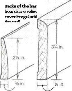
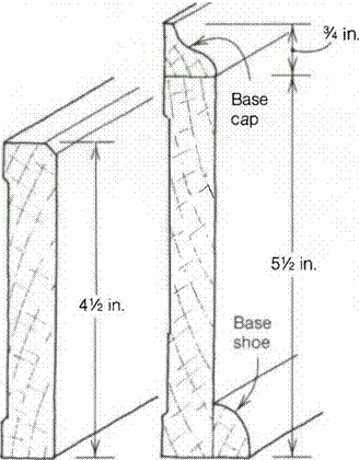
Casing hides the joint between the dry – wall and door jamb or window surround It comes in many styles, from 1 x square – edged stock in varying widths to milled casings (see the drawing above). When casing doors, I buy 14-ft. lengths to cut down on waste. Sometimes door casing is available in 7-ft. piecesthat have a 45° miter already cut on one end. Like exterior casings, doors and windows can be either picture-framed (with 45° miters at the corners) or wider trim can

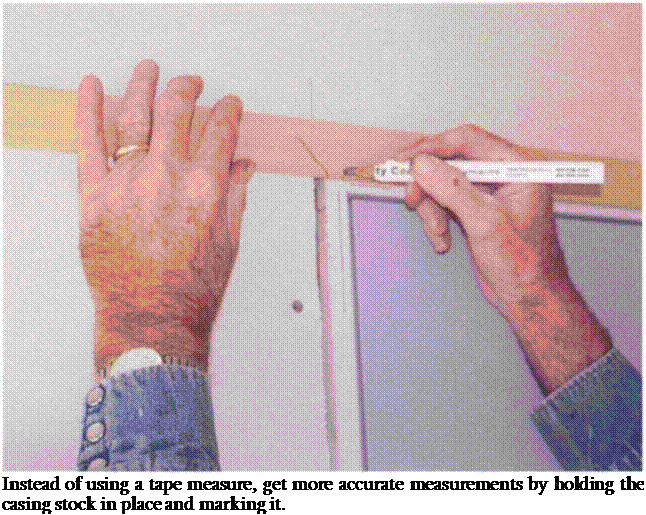
Подпись: Instead of using a tape measure, get more accurate measurements by holding the casing stock in place and marking it.

be butt jointed. I generally nail casing back from the edge of the jamb about 3/i6 in. to leave a reveal.

Reveals make life easier for a carpenter. When wood pieces are nailed flush, they absorb moisture or dry out, moving back and forth in the process, so that flush pieces seldom stay flush. Carpenters learned long ago to step casings back from the door edge 3/ie in. or so. This creates an attractive shadow line and makes it hard to see variations.

Install the side casings first. The short point of the miter should stop 3/ie in. past the top of the inside edge of the head door jamb or window surround. Rather than use a tape measure, hold and mark the casing stock in place (see the photo above). Mark the 3/ie-in. reveal from the inside edge of the jamb in several places and nail the casing into the wall and the jamb with a pair of 6d
finish nails about every 1 б in. Don’t drive these nails home like a 16d framing nail, but letthem stick up (proud) slightly above the face of the wood, setting them later with a nailset so they can be hidden with putty in preparation for painting. Or you can use an air nailer that drives and sets finish nails. If you are using hardwood casing, you may have to predrill to avoid splits.

Once the side pieces are in place, it’s easy to find the length of the top piece. Cut a miter on one end of the top piece and match it to the miters on the side pieces to see if the cut is accurate. Then hold it in place to mark the location of the second miter. Before nailing it in place, a dab of glue in the joints will make for a long-lasting miter joint.

A window apron, usually made from casing material, is nailed under the stool to hide the joint between drywall and sill. Measure across the window casing

Installing casing
Installing casing

from outside to outside to get the length of the apron. There are several ways to finish off the end of aprons.

You can cut them square or give them a 15° back cut and nail them directly below the windowsill.

Install the interior-door hardware

Interior-door handles and locks are installed in essentially the same manner as those used on exterior doors. Most interior doors just require a handle and a latch, or what is com­monly known as a passage-door lockset. However, for bedroom and bathroom doors, you may want a privacy lock—an interior lockset that locks when you push or turn a button.

Install the bathroom hardware and fixtures

One of your primary concerns when installing fixtures in a bathroom is to make sure they won’t come loose in a month or two. A toilet paper holder, for example, should be screwed into solid wood and not into drywall alone. This is why we installed backing in the bath­
room walls when we framed the walls (see chapter 4). if, for whatever reason, there is no backing in the wall, try to mount items by screwing them into studs. If you simply can’t avoid fastening into drywall alone, use an expansion, or toggle, bolt that goes through the drywall and opens in the back.

A recessed medicine cabinet is installed in the hole left in the drywall, which is usually directly over the sink. If the cabinet is surface mounted, position it so the bottom edge is 4 ft. from the floor, then screw it into studs or backing.

The toilet-paper holder should be screwed either into backing near the toilet, at 24 in. o. c. above the floor, or into a nearby vanity cabinet at the same height. Towel bars should be installed near the tub and vanity at 54 in. o. c. above the floor (see the photo on p. 272). If you want to install a toothbrush and cup holder, they should be located 4 in. above the

Подпись: INSTALL BATHROOM FITTINGS AT THE RIGHT HEIGHT. The toilet-paper holder should be about 24 in. from the floor. Towel bars, which are usually placed near the tub and vanity, should be 54 in. from the floor. [Photo by Roe A. Osborn, courtesy Fine Homebuilding magazine, ® The Taunton Press, Inc.] Подпись: Helping HandПодпись: Childproof latches are inexpensive lifesavers. If you plan to store poisonous compounds, such as drain cleaner and bleach, under the sink or in any base cabinet, keep them out of children's hands by installing childproof latches on cabinet doors. sink or 40 in. from the floor. It’s also a good idea to put a small clothes hook or two on the back of the bathroom door.

Various types of shower curtain rods can be installed in different ways. I like the ones that mount in sockets that are screwed into wall studs, much like the pole in a clothes closet. Or you can use the type of rod that is held by pressure between the two walls that surround the tub-shower. Cut the rod to length with a hacksaw, locate it just above the top of the shower walls, then expand it until it holds itself in place. Don’t forget to hang a beautiful shower curtain to add some color to your bathroom.

STEP 2 Select and Install the Finish Flooring

Things are looking good. The house is painted; the doors, cabinets, and countertops have been installed; and all your faucets and light switches are working. But one major transfor­mation remains—the finish flooring.

Installing finish flooring is one of the last jobs to do or have done, and for good reason. Now that you’re down to the detail work, fewer workers will be coming through the house, so there is less chance that the flooring will be damaged. There are many options, even for affordable homes, so this is a great opportunity to make choices that express your personal style.