Second-Order Reliability Methods
By the AFOSM reliability method, the design point on the failure surface is identified. This design point has the shortest distance to the mean point of the stochastic basic variables in the original space or to the origin of standardized normal parameter space. In the AFOSM method, the failure surface is locally approximated by a hyperplane tangent to the design point using the first-order terms of the Taylor series expansion. As shown in Fig. 4.14, second – order reliability methods (SORMs) can improve the accuracy of calculated reliability under a nonlinear limit-state function by which the failure surface is approximated locally at the design point by a quadratic surface. Literature on the SORMs can be found elsewhere (Fiessler et al., 1979; Shinozuka, 1983;
Breitung, 1984; Ditlevsen, 1984; Naess, 1987; Wen, 1987; Der Kiureghian et al., 1987; Der Kiureghian and De Stefano, 1991). Tvedt (1983) and Naess (1987) developed techniques to compute the bounds of the failure probability. Wen (1987), Der Kiureghian et al. (1987), and others demonstrated that the second – order methods yield an improved estimation of failure probability at the expense of an increased amount of computation. Applications of second-order reliability analysis to hydrosystem engineering problems are relatively few as compared with the first-order methods.
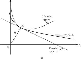
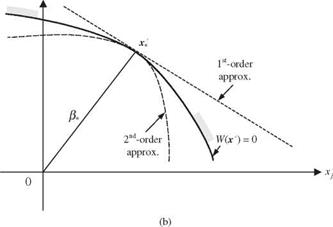
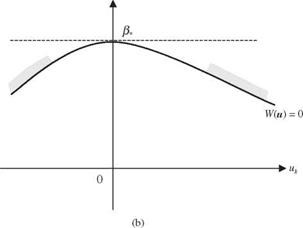
In the following presentations of the second-order reliability methods, it is assumed that the original stochastic variables X in the performance function W (X) have been transformed to the independent standardized normal space by Z’ = T (X), in which Z’ = (Z1, Z’2,…, Z’K) is a column vector of independent standard normal random variables. Realizing that the first-order methods do not account for the curvature of the failure surface, the first-order failure probability could over – or underestimate the true pf depending on the curvilinear nature of W(Z’) at z*. Referring to Fig. 4.15a, in which the failure surface is convex toward the safe region, the first-order method would overestimate the failure probability pf, and, in the case of Fig. 4.156, the opposite effect would result. When the failure region is a convex set, a bound ofthe failure probability is (Lind, 1977)
Ф(-&) < Pf < 1 – Fxf(&) (4.84)
in which в* is the reliability index corresponding to the design point z *, and Fx|(e+) is the value of the xK CDF with K degrees of freedom. Note that the upper bound in Eq. (4.84) is based on the use of a hypersphere to approximate the failure surface at the design point and, consequently, is generally much more conservative than the lower bound. To improve the accuracy of the failure – probability estimation, a better quadratic approximation of the failure surface is needed.
4.6.1 Quadratic approximations of the performance function
At the design point z * in the independent standard normal space, the performance function can be approximated by a quadratic form as
W (Z’) « 8 z (Z’ – z i) + ± (Z’ – z( / Gz> (Z’ – z:)
 |

|
xk
|
|
xk
Figure 4.15 Schematic sketch of nonlinear performance functions: (a) convex performance function (positive curvature); (b) concave performance function (negative curvature). |
in which sz’t = Vz W (z 7+) and GZt = V|, W (z ^) are, respectively, the gradient vector containing the sensitivity coefficients and the Hessian matrix of the performance function W (Z’) evaluated at the design point z The quadratic approximation by Eq. (4.85) involves cross-product of the random variables. To eliminate the cross-product interaction terms in the quadratic approximation, an orthogonal transform is accomplished by utilizing the symmetric square
nature of the Hessian matrix:
![]() Gzi = Al W (г 1) =
Gzi = Al W (г 1) =
Byway of spectral decomposition, Gz>t = V tGt KGt VG,, with VG, and AG, being, respectively, the eigenvector matrix and the diagonal eigenvalue matrix of the Hessian matrix Gz,. Consider the orthogonal transformation Z" = VGt Z’ by which the new random vector Z" is also a normal random vector because it is a linear combination of the independent standard normal random variables Z’. Furthermore, it can be shown that
E (Z") = 0
Cov( Z") = Cz« = E (Z "Z"l) = V G, Cz VGt = V G, VGt = I
This indicates that Z" is also an independent standard normal random vector. In terms of Z", Eq. (4.85) can be expressed as
W (Z") « 8 z, (Z" – г.) + 1(Z" – г,) Ag. (Z" – г,0
K 1 K
= ^2 8z’l, k(Zk – г,,k) + ^53 ^k(Zk7 – г,,k)2 = 0 (4.86)
k=i k=i
in which sz"tk is the kth element of sensitivity vector sz« = V tGt sz, in г "-space, and X’k is the kth eigenvalue of the Hessian matrix Gz,.
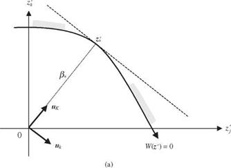
In addition to Eqs. (4.85) and (4.86), the quadratic approximation of the performance function in the second-order reliability analysis can be expressed in a simpler form through other types of orthogonal transformation. Referring to Eq. (4.85), consider a K x K matrix H with its last column defined by the negativity of the unit directional derivatives vector d* = – at = – sz>t /1sz, | evaluated at the design point г,, namely, H = [A1, h2,…, hK-1, d,], with hk being the kth column vector in H. The matrix H is an orthonormal matrix because all column vectors are orthogonal to each other; that is, ht hk = 0, for j = k, hkd, = 0, and all of them have unit length Ht H = HHt = I. One simple way to find such an orthonormal matrix His the Gram-Schmid orthogonal transformation, as described in Appendix 4D. Using the orthonormal matrix as defined above, a new random vector U can be obtained as U = Ht Z’. As shown in Fig. 4.16, the orthonormal matrix H geometrically rotates the coordinates in the г ‘-space to a new ы-space with its last uK axis pointing in the direction of the design point г,. It can be shown easily that the elements of the new random vector U = (U1, U2,…, UK)t remain to be independent standard normal random variables as Z’.
|
UK |
|
Figure 4.16 Geometric illustration of orthonormal rotation. (a) Before rotation (b) After rotation. |
Knowing z * = в* d *, the orthogonal transformation using H results in
u* = H1 z* = H1 (e*d*) = в*H1 d* = в*(0, 0,… ,1)
indicating that the coordinate of the design point in the transformed u-space is (0, 0, …, 0, в*). In terms of the new u-coordinate system, Eq. (4.2) can be expressed as
W (U) « s U* (U – u*)+hu – uj H1 Gz-* H(U – u*) = 0 (4.87)
2
where su, = H1 szt, which simply is
s U, = (s z, hi, s Z h2> •••>s Z hK-i, s z, d,)
= ( |sZ.,d, hi, |sz,|d, h2,|sz,|d„h^-i, -|sz,|d, d,)
= (0,0, …,0,-|s z,|) (4.88)
After dividing |s z, | on both sides of Eq. (4.4), it can be rewritten as
W(U) « в, U k + 1(U – u,)‘ A,(U – u,) = 0 (4.89)
in which A, = Hг Gz, H/ |s z,|. Equation (4.6) can further be reduced to a parabolic form as
W(U) « в, – Uk + 1U1 A, U = 0 (4.90)
2
where U = (U1, U 2, …, UK-1) and A, is the (K – 1)th order leading principal submatrix of A, obtained by deleting the last row and last column of matrix
A.
To further simplify the mathematical expression for Eq. (4.7), an orthogonal transformation is once more applied to U as U = У1А U with being the eigenvector matrix of A, satisfying A, = Уд Лд, Уд,, in which Aa, is the diagonal eigenvalues matrix of A,. It can easily be shown that the elements of the new random vector U s are independent standard normal random variables. In terms of the new random vector U’, the quadratic term in Eq. (4.7) can be rewritten as
W(U’, Uk) « в, – Uk + iUЛд, U’
1 K-1
= в, – Uk + KkUk2 = 0 (4.91)
2 k=1

where к’s are the main curvatures, which are equal to the elements of the diagonal eigenvalue matrix Лд, of matrix A,. Note that the eigenvalues of A, are identical to those of Gz, defined in Eq. (4.2). This is so because A, = H1 Gz, H is a similarity transform. Therefore, the main curvatures of the hyperparabolic approximation of W(Z’) = 0 are equal to the eigenvalues of A,.
where фк(z 0 is the joint PDF of K independent standard normal random variables. This type of integration is called the Laplace integral, and its asymptotic characteristics have been investigated recently by Breitung (1993).
Once the design point z* is found and the corresponding reliability index в* = z * is computed, Breitung (1984) shows that the failure probability based on a hyperparabolic approximation of W(Z0, Eq. (4.92), can be estimated asymptotically (that is, в* ^-<x>) as
K-1
Pf « Ф(-в,) Ц(1 + вк)-1/2 (4.93)
k=1
where Kk, k = 1,2,…, K — 1, are the main curvatures of the performance function W(Z’) at z*, which is equal to the eigenvalues of the (K — 1) leading principal submatrix of A * defined in Eq. (4.90). It should be pointed out that owing to the asymptotic nature of Eq. (4.93), the accuracy of estimating pf by it may not be satisfactory when the value of в* is not large.
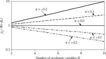
Equation (4.93) reduces to pf = Ф(—в*) if the curvature of the performance function is zero. A near-zero curvature of W (Z’) in all directions at the design point implies that the performance function behaves like a hyperplane around z*. In this case, W(Z’) at z* can be described accurately by the first-order expansion terms, and reliability corresponds to the first-order failure probability. Figure 4.17 shows the ratio of second-order failure probability by Eq. (4.93) to the first-order failure probability as a function of main curvature and number of stochastic variables in the performance function. It is clearly shown in Fig. 4.17a that when the limit-state surface is convex toward the failure region with a constant positive curvature (see Fig. 4.15a), the failure probability estimated by the first-order method is larger than that by the second-order methods. This magnitude of the overestimation increases with the curvature
|
Figure 4.17 Comparison of the second-order and first-order failure probabilities for performance function with different curvatures. |
and the number of stochastic basic variables involved. On the other hand, the first-order methods yield a smaller value of failure probability than the second – order methods when the limit-state surface is concaved toward the safe region (see Fig. 4.156), which corresponds to a negative curvature. Hohenbichler and Rackwitz (1988) suggested further improvement on Breitung’s results using the importance sampling technique (see Sec. 6.7.1).
In case there exists multiple design points yielding the same minimum distance в*, Eq. (4.93) for estimating the failure probability pf can be extended as
in which J is the number of design points with в* = z *1| = |z *2| = ■ ■ = |z * J |, and Kk, j is the main curvature for the kth stochastic variables at the j th design point.
The second-order reliability formulas described earlier are based on fitting a paraboloid to the failure surface at the design points on the basis of curvatures. The computation of failure probability requires knowledge of the main curvatures at the design point, which are related to the eigenvalues of the Hessian matrix of the performance function. Der Kiureghian et al. (1987) pointed out several computational disadvantages of the paraboloid-fitting procedure:
1. When the performance function is not continuous and twice differentiable in the neighborhood of the design point, numerical differencing would have to be used to compute the Hessian matrix. In this case, the procedure may be computational intensive, especially when the number of stochastic variables is large and the performance function involves complicated numerical algorithms.
2. When using numerical differencing techniques for computing the Hessian, errors are introduced into the failure surface. This could result in error in computing the curvatures.
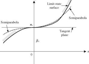
3. In some cases, the curvatures do not provide a realistic representation of the failure surface in the neighborhood of design point, as shown in Fig. 4.18.
To circumvent these disadvantages of curvature-fitting procedure, Der Kiureghian et al. (1987) proposed an approximation using a point-fitted paraboloid (see Fig. 4.18) by which two semiparabolas are used to fit the failure surface in such a manner that both semiparabolas are tangent to the failure surface at the design point. Der Kiureghian et al. (1987) showed that one important advantage of the point-fitted paraboloid is that it requires less computation when the number of stochastic variables is large.

|
|
|
|
|
|
|


Leave a reply