Lognormal distribution
The lognormal distribution is a commonly used continuous distribution for positively valued random variables. Lognormal random variables are closely related to normal random variables, by which a random variable X has a lognormal distribution if its logarithmic transform Y = ln(X) has a normal distribution with mean xln x and variance оЩx. From the central limit theorem, if a natural process can be thought of as a multiplicative product of a large number of an independent component processes, none dominating the others, the lognormal
distribution is a reasonable approximation for these natural processes. The PDF of a lognormal random variable is
|
|
||
|
|||

which can be derived from the normal PDF. Statistical properties of a lognormal random variable in the original scale can be computed from those of log – transformed variables as
Mx — A — exp ^ Mln x + j (2.66a)
el — МІ [exp (°-l2nx) – 1] (2.66b)
^2 — exp (ol2nx) – 1 (2.66c)
Kx — ^3 + 3^x (2.66d)
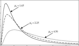
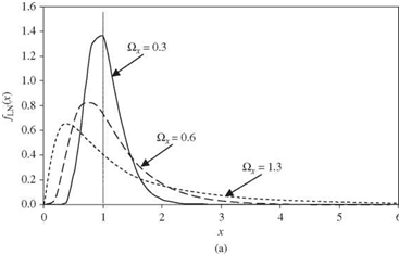
From Eq. (2.66d), one realizes that the shape of a lognormal PDF is always positively skewed (Fig. 2.19). Equations (2.66a) and (2.66b) can be derived easily by the moment-generating function (Tung and Yen, 2005, Sec. 4.2). Conversely, the statistical moments of ln(X) can be computed from those of X by
It is interesting to note from Eq. (2.67b) that the variance of a log-transformed variable is dimensionless.
In terms of the L-moments, the second-order L-moment for a two – and three – parameter lognormal distribution is (Stedinger et al., 1993)
(2.68)
in which erf( ) is an error function the definitional relationship of which, with
Ф(г) is
2 fx 2 fx
erf(x) — ^= e~“2 du — e-Z/2 dz — 2Ф(^/2x) – 1 (2.69)
Vn Jo vn Jo
Hence the L-coefficient of variation is r2 — 2Ф(о1пx Д/2) – 1. The relationship between the third- and fourth-order L-moment ratios can be approximated by the following polynomial function with accuracy within 5 x 10⁻⁴ for | r2 | < 0.9 (Hosking, 1991):
T4 — 0.12282 + 0.77518т32 + 0.12279т34 – 0.13638t36 + 0.11386r38 (2.70)


 |
0.6
0.5
z
i – J
0.3 0.2 0.1 0
Since the sum of normal random variables is normally distributed, the product of lognormal random variables also is lognormally distributed (see Fig. 2.15). This useful reproductive property of lognormal random variables can be stated as if X1,X2,…,XK are independent lognormal random variables, then W = b0nK= 1 Xbb has a lognormal distribution with mean and variance as
K K
M-ln w = ln(b0) + 53 bk M-lnXk °ln w =53 bk alnxk
к = 1 k = 1
In the case that two lognormal random variables are correlated with a correlation coefficient pXyy in the original scale, then the covariance terms in the
log-transformed space must be included in calculating аЩ w. Given px, y, the correlation coefficient in the log-transformed space can be computed as
Corr(ln X, lnY) = Pln x, ln y = , ln(1 + Px’yUx Uy) (2.71)
^ln(1 + Д2) x ln(1 + Д2)
Derivation of Eq. (2.71) can be found in Tung and Yen (2005).
Example 2.18 Re-solve Example 2.17 by assuming that the annual maximum flood magnitude in the river follows a lognormal distribution.
Solution (a) Since Q has a lognormal distribution, ln( Q) is normally distributed with a mean and variance that can be computed from Eqs. (2.67a) and (2.67b), respectively, as
Qq = 4000/6000 = 0.667 afn Q = ln(1 + 0.66 72) = 0.3 68 MlnQ = ln(6000) – 0.368/2 = 8.515
The probability of the annual maximum flood magnitude exceeding 10,000 ft3/s is P (Q > 10, 000) = P [ln Q > ln(10, 000)]
= 1 – P [Z < (9.210 – 8.515)/V0.368]
= 1 – Ф(1.146) = 1 – 0.8741 = 0.1259
(b) A 100-year flood qw0 represents the event the magnitude of which corresponds to P(Q > <7100) = 0.01, which can be determined from
P(Q < 7100) = 1 – P(Q > 7100) = 0.99
because P(Q < 7100) = P [ln Q < ln(q100)]
= P {Z < [ln(7100) – Mln Q]/oln Q1
= P{Z < [ln(q100) – 8.515]/V0.368}
= Ф{[1п(7100) – 8.515]Д/0.368} = 0.99 From Table 2.2 or Eq. (2.64), one can find that Ф(2.33) = 0.99. Therefore,
[ln(q100) – 8.5151Л/0.368 = 2.33
which yields ln(q100) = 9.9284. The magnitude of the 100-year flood event then is q100 = exp(9.9284) = 20, 500 ft3/s.


Leave a reply