Importance sampling technique

The importance sampling technique concentrates the distribution of sampling points in the part of the domain that is most “important” for the task rather than spreading them out evenly (Marshall, 1956). Refer to the problem of evaluating an integral in Eq. (6.49) by the sample-mean method. The importance sampling technique attempts to generate M sampling points to reduce the variance of G given by Eq. (6.61).

Rubinstein (1981) showed that the PDF fx(x) that minimizes Eq. (6.61) can be obtained as

|g (x)| / |g (x)| dx
fx(x)	(6.72)
Although Eq. (6.72) indicates that the weighing function fx(x) is a function of / |g (x)| dx, which is practically equivalent to the integral sought, however, it is not completely useless. Equation (6.72) implies that if is fx(x) is chosen to have a similar shape as |g (x)|, considerable reduction in variance of the simulation results can be achieved. However, in practical implementations of this technique, consideration must be given to the tradeoffbetween the desired error reduction and the difficulties of sampling from fx (x), especially when |g (x)| is not well behaved.
Example 6.9 Repeat Example 6.6 using the importance sampling technique with n = 2000. The PDF selected is a trapezoidal distribution with a PDF defined as ht(t) = 0.006 — b x t for 0 < t < 200
where b is the slope of the dashed line shown in Fig. 6.12. Compare the efficiency of the technique under this distribution with that in Examples 6.6 and 6.7.
Solution Using the importance sampling method with the trapezoidal PDF indicated earlier, evaluation of the pump failure probability can be expressed as
(i)

ft (t) Figure 6.12 Importance sampling for integration in Example 6.9.

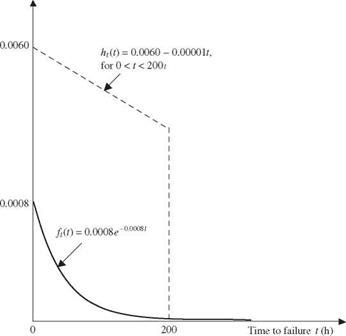
From condition (i), the coefficient b can be obtained easily as b = 0.00001. Substituting b = 0.00001 into ht(t), one can verify that condition (ii) is also satisfied. Therefore, ht(t) = 0.006 — 0.00001 x t is a legitimate PDF in 0 < t < 200. To generate random variates from ht(t), the CDF-inverse method can be used because the CDF of ht(t) can be obtained easily as

Ht(T) = U = (0.006 — 0.00001t) dt = 0.006T — ^°-002001) T 2

Solving for T in terms of U, one obtains

in which a = 0.006 and b = 0.00001. Based on the boundary conditions of a CDF, that is, Ht(t = 0) = 0 and Ht(t = 200) = 1, the only valid expression for T from ht(t) is

T 2a — V 4a2 — 8bU

= 2b

Hence the preceding equation can be used to generate random variates from ht(t). The algorithm for this example can be outlined as follows:

1. Generate n standard uniform random variates ui from U(0, 1).

2. Compute ti according to Eq. (6.73), yielding n random variates from ht(t) = 0.006 —

0. 00001t, 0 < t < 200.

3. Estimate the pump failure probability as

0.0008e-0’0008ti 0.006 — 0.00001ti)

ft (ti) ht (ti)

i=1

i=1

4. To assess the error associated with the estimated pump failure probability by the preceding equation, compute the following quantity:

(6.74)

2

pZ

Using this algorithm, the estimated pump failure probability is pf = 0.14767, whereas the exact failure probability is 0.147856. The associated standard error can be computed as

sp f = 0.00023

Assuming normality for the estimated pump failure probability, the 95 percent confi­dence interval containing the exact risk pf is

pf ± 1.96spf = (0.14722,0.14813)

Comparing the solutions with those of Examples 6.6 and 6.7, it is observed that with the same n = 2000, the importance sampling method has a 0.126 percent error. The magnitude of error and the accuracy level are somewhat worse than the sample- mean procedure but are still far better than the hit-and-miss algorithm. The accuracy of the importance sampling technique depends on how ht(t) is specified. As can be observed from Problem 6.29, use of the exponential function for ft(t) improves the accuracy tremendously.