Determinations of availability and unavailability

Determination of the availability or unavailability of a system requires a full accounting ofthe failure and repair processes. The basic elements that describe such processes are the failure density function ft (t) and the repair density func­tion gt (t). In this section computation of the availability of a single component or system is described under the condition of an ideal supportability. That is, the availability, strictly speaking, is the inherent availability. Discussions of the subject matter for a complex system are given in Chap. 7.

Consider a specified time interval (0, t], and assume that the system is ini­tially in an operating condition at time zero. Therefore, at any given time in­stance t, the system is in an operating state if the number of failures and repairs w(0, t) are equal, whereas the system is in a failed state if the number of failures exceeds the number of repairs by one. Let NF (t) and Nr (t) be the random vari­ables representing the numbers of failures and repairs in time interval (0, t], respectively. The state of the system at time instance t, failed or operating, can be indicated by a new variable I (t) defined as

I (t) = Nf (t) — Nr(t) (5.45)

Note that I(t) also is a random variable. As described earlier, the indicator variable I (t) is binary by nature, that is,

1 if system is in a failed state

0 otherwise

Recall that the unavailability is the probability that a system is in the failed state, given that the system was initially operational at time zero. Hence the unavailability of a system is the probability that the indicator variable I (t) takes the value of 1, which is equal to the expected value of I (t). Accordingly,

U(t) = E [I (t)] = E [Nf (t)] — E [Nr(t)] = W(0, t) — Г(0, t) (5.46)

indicating that the unavailability is equal to the expected number of failures W(0, t) minus the expected number of repairs Г(0, t) in time interval (0, t]. The values of W(0, t) and Г(0, t) can be computed by Eqs. (5.43) and (5.44), respectively.

To compute W(0, t) and Г(0, t), knowledge of the unconditional failure in­tensity w(t) and the unconditional repair intensity y(t) is required. The un­conditional failure intensity can be derived by the total probability theorem as

w(t) = ft(t) +( y(t) ft(t — r) dr (5.47)

0

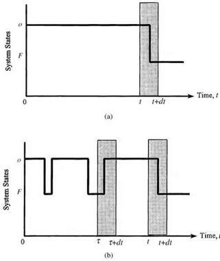
in which, on the right-hand side, the first term, ft (t), is for the case that the probability of failure is at time t, given that the system has survived up to time t; the second term accounts for the case that the system is repaired at time r < t and later fails at time t. This is shown in Fig. 5.18.

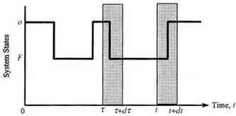
For the unconditional repair intensity y (t) one would need only to consider one possible case, as shown in Fig. 5.19. That is, the system is in an operating state at time t given that the system is operational initially and is in a failed state at time r < t. The probability that this condition occurs is

Y(t) = [ w(r)g(t — r) dr (5.48)

0

Figure 5.18 Two different cases for a system to be in a failed state during (t, dt]: (a) the system has been operational up to time t and failed during (t, t + dt), given that it was good at t = 0 and no repair has been done during (0, t); (b) the system has been operational up to time tand failed during (t, t + dt), given that it was good at t = 0 and was repaired at t = т. (After Henley and Kumamoto, 1981.)

Note that given the failure density ft(t) and the repair density gt(t), the un­conditional failure intensity w(t) and the unconditional repair intensity y(t) are related to one another in an implicit fashion, as shown in Eqs. (5.47) and (5.48). Hence the calculations of w(t) and y (t) are solved by iterative numerical integration. Analytically, the Laplace transform technique can be applied to derive w(t) and y(t) owing to the convolution nature of the two integrals.

Based on the unavailability and unconditional failure intensity, the condi­tional failure intensity g(t) can be computed as

w(t) 1 — U (t)	w(t) At)
g(t)	(5.49)

which is analogous to Eq. (5.3). For the repair process, the conditional repair intensity p(t), unconditional repair intensity y(t), and unavailability are re­lated as

p «> = ш (550)

The general relationships among the various parameters in the failure and repair processes are summarized in Table 5.4.

TABLE 5.4 Relationship among Parameters in Time-to-Failure Analysis Repairable systems Nonrepairable systems General relations A(t) + U (t) = 1 A(t) + U (t) = 1 A(t) > ps(t) A(t) = ps(t) U(t) < pf (t) U(t) = pf (t) w(t) = ft(t) + f ft(t — r)y(t) dr w(t) = ft (t) Y(t) = Jgt(t — r)w(r) dr Y(t) = 0 W(t1, t2) = Jw(r)dr W(t1, t2) = ps(t2) — ps(tx) r(t1, t2) = f Y(r)dr r(t1, t2) = 0 U(t) = W(0, t) — Г(0, t) U(t) = pf (t) !i(t) = w(t)/A(t) h(t) = ft (t)/ps(t) p (t) = y (t)/U (t) r(t) = 0 Stationary values MTBF = MTBR = MTTF + MTTR MTBF = MTBR = to 0 < A(to), U(to) < 1 A(to) = 0, U(to) = 1 0 < w(to), y(to) < to w(to) = 0, y(to) = 0 w(to) = y (to) w(to) = y (to) = 0 W(0, to) = Г(0, to) = to Remarks W(0, to) = 1, Г(0, to) = 0 w(t) = Mt), Y(t) = p(t) w(t) = Mt), Y(t) = p(t) = 0 Mt) = h(t), p(t) = r(t) p,(t) = h(t), p(t) = r (t) = 0 w(t) = ft(t), y(t) = gt(t) w(t) = ft(t), y(t) = gt(t) = 0 SOURCE : After Henley and Kumamoto (1981).

Example 5.12 For a given failure density function ft(t) and repair density function gt(t), solve for the unconditional failure intensity w(t) and the unconditional repair intensity y(t) by the Laplace transform technique.

Solution Note that the integrations in Eqs. (5.47) and (5.48) are in fact convolutions of two functions. According to the properties of the Laplace transform described in Appendix 5A, the Laplace transforms of Eqs. (5.47) and (5.48) result in the following two equations, respectively:

L[w(t)] = L[ ft(t)] + L[y(t)] x L[ ft(t)] (5.51a)

L[y(t)] = L[w(t)] x L[gt(t)] (5.51b)

in which L(-) is the Laplace transform operator. Solving Eqs. (5.51a) and (5.51b) simultaneously, one has

To derive w(t) and y(t), the inverse transform can be applied to Eqs. (5.52a) and (5.52b), and the results are

and

Example 5.13 (Constant failure rate and repair rate) Consider that the failure den­sity function ft(t) and the repair density function gt (t) are both exponential distribu­tions given as

ft(t) = Xe Xt for X > 0, t > 0

gt(t) = ne—qt for n > 0, t > 0

Derive the expressions for their availability and unavailability.

Solution The Laplace transform of the exponential failure density ft(t) is

/•TO /»ТО X

L[ ft(t)] = e-st ft(t) dt = X e-(s+X)t dt = ——————

Л J0 X +s

Similarly, L[gt(t)] = n/(n + s). Substituting L[ ft(t)] and L[gt(t)] into Eqs. (5.52a) and (5.52b), one has

(Л _X^( 1

X + n s f X + n s + X + n )

Taking the inverse transform for the preceding two equations, the results are

The availability A(t) then is

A(t) = 1 — U(t) = -^ + —e-(k+n)t к + n к + n

As the time approaches infinity (t ^ те), the system reaches its stationary condition. Then the stationary availability А(те) and unavailability U(те), are

А(те) =	n	1/k	MTTF	(5.60)
к + n	1/k + 1/n	= MTTF + MTTR
U (те) =	к	1/n	MTTR	(5.61)
к + n	1/k + 1/n	MTTF + MTTR

Other properties for a system with constant failure and repair rates are summarized in Table 5.5. Results obtained in this example also can be derived based on the Markov analysis (Henley and Kumamoto, 1981; Ang and Tang, 1984).

Strictly speaking, the preceding expressions for the availability are the inherent availability under the condition of an ideal supportability with which the mean time to support (MTTS) is zero. In the case that the failed system requires some time to respond and prepare before the repair task is undertaken, the actual availability is

MTTF

MTTF + MTTR + MTTS which, as compared with Eq. (5.60), is less than the inherent availability.

Repairable systems	Nonrepairable systems
Failure process
h(t) = X	h(t) = X
Ps (t) = e-Xt	Ps(t) = e-Xt
Pf (t) = 1 — e-Xt	Pf (t) = 1 — e-Xt
ft (t) = Xe-lt	ft (t) = Xe-Xt
MTTF = 1/X	MTTF = 1/X
Repair process
r (t) = n	r(t) = 0
Gt (t) = 1 — e-nt	Gt(t) = 0
gt (t) = ne-nt	gt (t) = 0
MTTR = 1/n	MTTR = to
Dynamic behavior of whole process
U(t) = X/(X + n)(1 — e-(X+n)t)	U(t) = 1 — e-Xt = Pf (t)
A(t) = n/(X + n) + X/(X + n)(1 — e-(x+n)t)	A(t) = e-Xt = Ps(t)
a(t) = Xn/(X + n) + X2/(X + n)(1 — e-(X+n)t)	w(t) = ft (t) = Xe-Xt
Y(t) = Xn/(X + n)(1 — e-(X+n)t)	Y(t) = 0
W(0, t) = Xnt/(X + n) + X2/(X + n)(1 — e-(X+n)t)	W(0, t) = Pf (t)
r(0, t) = Xnt/(X + n) — Xn/(X + n)2(1 — e-(X+n)t)	О II o’
Stationary values of whole process
U (to) = X/(X + n) = MTTR/(MTTF + MTTR)	U (to) = 1
A(to) = n/(X + n) = MTTF/(MTTF + MTTR)	A(to) = 0
ш(то) = Xn/(X + n) = 1/(MTTF + MTTR)	w(to) = 0
Y (to) = Xn/(X + n) = w(to)	Y (to) = 0

TABLE 5.5 Summary of the Constant Rate Model

SOURCE : After Henley and Kumamoto (1981).

Example 5.14 Referring to Example 5.12, with exponential failure and repair density functions, determine the availability and unavailability of the pump.

Solution Since the failure density and repair density functions are both exponential, the unavailability U(t) of the pump, according to Eq. (5.58), is

The availability A(t) then is

A(t) = 1 — U(t) = 0.9615 + 0.03846e-00208t

The stationary availability and unavailability are

4 MTTF 1/X 1250

A(to) = MTTF + MTTR = I/m/n = 1250 + 50 = a96154 U(to) = 1 — A(to) = 1 — 0.96154 = 0.03846

TABLE 5.6 Operation Properties of the Laplace Transform on a Function Property Function Variable Laplace transform Standard fx ( x) X Lx(s) Scaling fx (ax) X a-1 Lx (s/a) Linear afx(x) X aLx (s) Translation-1 eaxfx (x) X Lx (s + a) Translation-2 fx (x — a) X easLx(s), x > a

Appendix 5A: Laplace Transform*

The Laplace transforms of a function fx(x) are defined, respectively, as

In a case where f x(x) is the PDF of a random variable, the Laplace transform defined in Eqs. (5A.1) can be stated as

Lx(s) = E [esX] for x > 0 (5A.2)

Useful operational properties of the Laplace transform on a PDF are given in Table 5.6. The transformed function given by Eq. (5A.1) of a PDF is called the moment-generating function (MGF) and is shown in Table 5.7 for some com­monly used probability distribution functions. Some useful operational rules relevant to the Laplace transform are given in Table 5.8.

‘Extracted from Tung and Yen (2005).

Uniform	Eq. (2.100)	ee
	(b — a)s
Normal	Eq. (2.58)	exp(/u, s — 0.5s
Gamma	Eq. (2.72)		1/в	a
	[(1/в) — s
Exponential	Eq. (2.79)		1/в
(1/в)—s
Extreme value I (max)	Eq. (2.85)	e4 sr(1 — в s)
Chi-square	Eq. (2.102)	(1 — 2s)—K/2

TABLE 5.7 Laplace Transform (Moment-Generating Functions) of Some Commonly Used Distribution Functions

Distribution

PDF Laplace transform

TABLE 5.8 Operational Rules for the Laplace Transform

W = cX Lw(s) = Lx(cs), c = a constant.

W = c + X Lw(s) = ecsLx(s), c = a constant.